14 Simple Regression

In this chapter, you’ll find instructions for fitting simple regression models, where there is a single predictor variable used to model a response.

For more general scenarios, including fitting simple or multiple linear regression models with diagnostic tools, model selection procedures, and additional fitting methods, please refer to Chapter 15.

To specifically fit a simple regression model, use the function Simple Regression, available under the Analytics toolbox and from the Linear Regression dropdown menu.

14.1 Specifying Data and Model

Figure 14.1 shows the dialog for the Simple Regression function. To fit a simple regression model, select a dataset from the Dataset dropdown. Then, select the predictor and response variables from the Predictor (x) and Response (y) dropdown menus, respectively. After selecting these, click the Preview icon to view your results. By default, the output includes the model summary, coefficients, and R-squared and correlation statistics. It also includes a scatterplot of the predictor and response variables with the fitted regression line, and residuals plotted against the fitted values.

14.1.1 Transforming predictor or response

You can transform either your predictor or response variable by directly typing the transformation into the corresponding dropdown menu. For example, if your dataset includes a variable called Height, and you wish to use its logarithm as your response, type log(Height) into the Response (y) field. The predictor variable can be transformed similarly.

14.1.2 Specifying a model without an intercept

By default, a simple regression model that you fit includes an intercept. To specify a model without an intercept (i.e., forcing the intercept to be zero), add a -1 next to the predictor variable in the Predictor (x) dropdown. For example, if your predictor variable is age, you can enter either age - 1 or -1 + age.

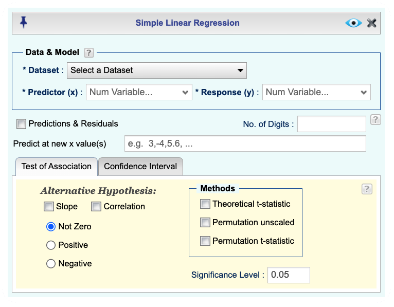
Figure 14.1: Simple Regression Basics dialog

14.2 Predictions and Residuals

When fitting a simple regression model, you can obtain predicted values and residuals based on the observed data. This is done by checking the Predictions & Residuals (Observed data) checkbox in the dialog box. This will include the predicted values and residuals in your output. In order to obtain predicted values and residuals, check the Predictions & Residuals checkbox in the dialog box. This will include the predicted values and residuals based on the observed data in your output. In addition, you can obtain predictions for new values by typing in values in the Predict at new x value(s) textbox. The values should be separated by commas. For example, if you want to predict the response for predictor values of 1, 2, and 3, you would enter 1, 2, 3 in the textbox.

14.3 Testing the Association between Predictor and Response

To test the association between the predictor and response variables, select either the Slope or Correlation checkbox (or both) in the dialog box. Selecting these will perform hypothesis tests for the slope and/or the correlation coefficient, providing p-values and confidence intervals.

To perform these tests, you must select at least one of the available testing methods: a theory-based approach (t-test) or permutation tests, by checking the corresponding boxes in the dialog.

You can also specify the type of test for the slope by selecting one of the following options:

• Not zero: Tests whether the slope is different from zero.
• Positive: Tests whether the slope is greater than zero.
• Negative: Tests whether the slope is less than zero.

The output will include the p-values and confidence intervals for the tests you have selected.

14.4 Confidence Intervals

Figure 14.2 shows the tab Confidence Interval in the Simple Regression dialog. This dialog allows you to specify the confidence level for the confidence intervals of the slope, correlation, as well as the prediction intervals for new observations or confidence intervals for fitted values.

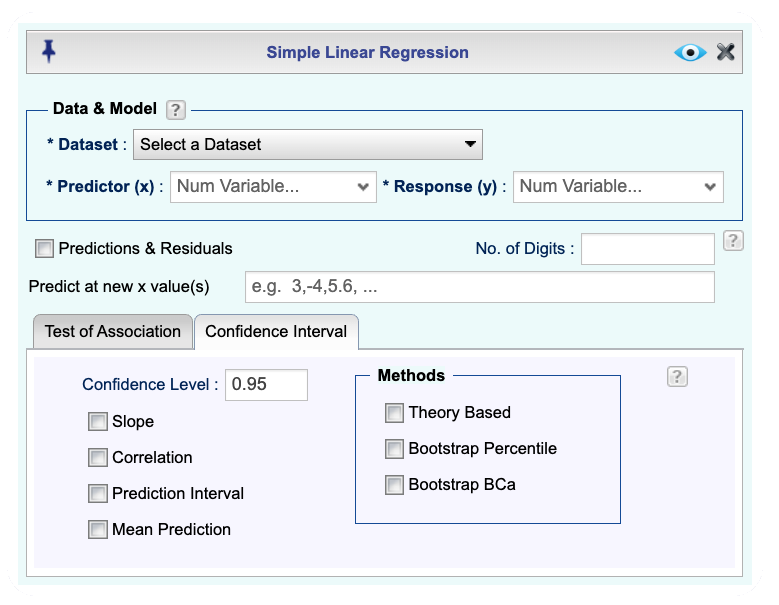
Figure 14.2: Simple Regression Confidence Interval dialog

14.5 An Example of Fitting a Simple Regression Model

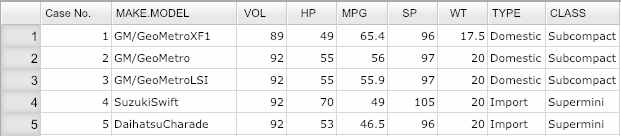
The follwowing is an example of fitting a simple regression model in Rguroo. The example uses the cardata dataset, which is available in the Rguroo dataset repository called Rguroo Users Guide. You can import this dataset into your Rguroo account using the command cardata. The output for the example is shown in Figure 14.3.

Instructions for fitting a s simple linear regression model in Rguroo:

1. Use a dataset in your Rguroo account or recreate the example below by importing the cardata dataset from the Rguroo dataset repository called Rguroo Users Guide into your account.

Click here to see a portion of the dataset.

2. Open the Analytics toolbox on the left-hand side of the Rguroo window. Use the Analysis dropdown menu and choose Linear Regression —> Simple Regression. This will open the Simple Regression dialog box (see Figure 14.3)

3. In the Data section, select a Dataset. Then select your predictor and response variables from the Predictor (x) and Response (y) dropdowns.

4. (Optional) You can obtain predicted values and residuals by selecting the Predictions & Residuals (Observed data) checkbox. Moreover, you can get predictions for new values and perform tests of hypotheses about correlation and slope and obtain confidence intervals for parameters and mean predictions and prediction intervals using both theory-based and bootstrap methods.

5. Click the Preview icon to view the result.

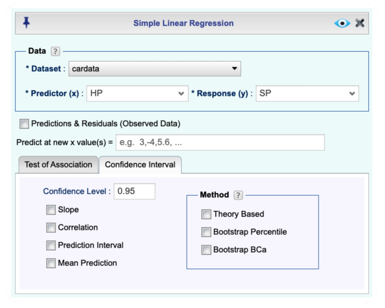
Figure 14.3: Simple regression dialog