19 Time Series Analysis

19.1 Time Plot

Instructions to create a time plot

1. Use a dataset in your Rguroo account or recreate the example below by importing the AirPassengers dataset from the Rguroo dataset repository called R Datasets into your account.

Click here to see a portion of the dataset.

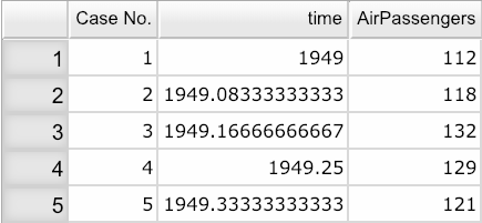
2. Open the Analytics toolbox on the left-hand side of the Rguroo window. Click on the Analysis dropdown menu and choose the Time Series function (see Figure 19.1).

3. Select your dataset from the Dataset dropdown menu. In this example, we select the AirPassengers dataset.

4. From the Numerical Variables section, select and drag the variable AirPassengers to the Selected column.

5. (Optional) Under the Time Specification section, from the Type dropdown, select the time frequency of your data (yearly, quarterly, monthly, daily, hourly, by minute or seconds). The AirPassengers data are monthly, so we select Month from the Type dropdown menu. Then set an appropriate start month and year for the data. The AirPassengers data starts from January 1949, so set Year to \(\tt{1949}\) and Month to \(\tt{1}\).

6. In the section Time Series Plot, select the Lines checkbox and optionally the Points checkbox.

7. Click the Preview icon to view the graph.

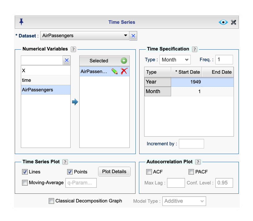
Figure 19.1: Time Series dialog for time plot.

19.2 Moving Average Plot

1. Use a dataset in your Rguroo account or recreate the example below by importing the AirPassengers dataset from the Rguroo dataset repository called R Datasets into your account (see Figure 19.2).

Click here to see a portion of the dataset.

2. Open the Analytics toolbox on the left-hand side of the Rguroo window. Click on the Analysis dropdown menu and choose the Time Series function.

3. Select your dataset from the Dataset dropdown menu. In this example, we select the AirPassengers dataset.

4. From the Numerical Variables section, select and drag the variable AirPassengers to the Selected column.

5. (Optional) Under the Time Specification section, from the Type dropdown, select the time frequency of your data (yearly, quarterly, monthly, daily, hourly, by minute or seconds). The AirPassengers data are monthly, so we select Month from the Type dropdown menu. Then set an appropriate start month and year for the data. The AirPassengers data starts from January 1949, so set Year to \(\tt{1949}\) and Month to \(\tt{1}\).

6. In the section Time Series Plot, select the Lines and Moving Average checkbox.

7. In the text field to the right of Moving-Average labeled q-Param, enter an integer value equal to the desired number of periods to calculate the moving average over.

8. Click the Preview icon to view the graph.

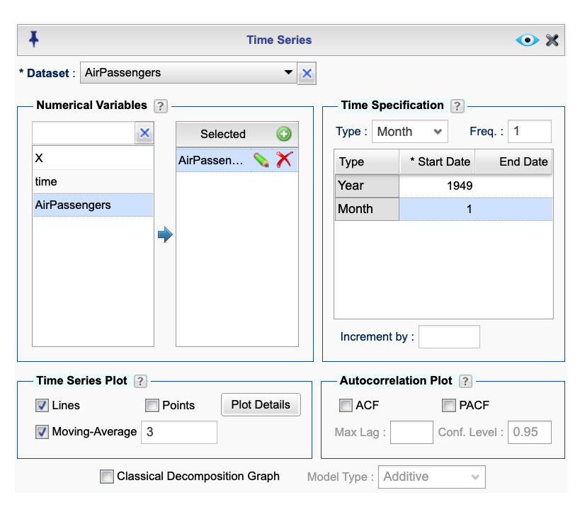
Figure 19.2: Time Series dialog for moving average plot.

19.3 Exponential Smoothing

Instructions to create an exponential smoothing plot in Rguroo

1. Use a dataset in your Rguroo account or recreate the example below by importing the USAccDeaths dataset from the Rguroo dataset repository called R Datasets into your account.

Click here to see a portion of the dataset.

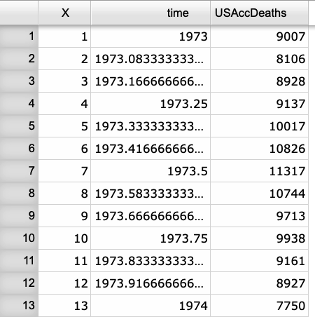
2. Open the Analytics toolbox on the left-hand side of the Rguroo window. Click on the Analysis dropdown menu and choose the Time Series function (see Figure 19.3) .

3. Select your dataset from the Dataset dropdown menu. In this example, we select the USAccDeaths dataset.

4. From the Numerical Variables section, select and drag the variable USAccDeaths to the Selected column.

5. (Optional) Under the Time Specification section, from the Type dropdown, select the time frequency of your data (yearly, quarterly, monthly, daily, hourly, by minute or seconds). The USAccDeaths data are monthly, so we select Month from the Type dropdown menu. Then set an appropriate start month and year for the data. The USAccDeaths data starts from January 1, 1973 so set Year to \(\tt{1973}\) and Month to \(\tt{1}\).

6. Click on the button to open the modeling dialog.

7. In the Methods and Forecasting dialog under the Method section, check Exponential and Graph.

8. In the text field to the right of Exponential, optionally enter an Alpha value between 0 and 1. If a value is not specified, a default value will be chosen by Rguroo. We use a value of 0.5 for Alpha in this example.

9. Click the Preview icon to view the graph.

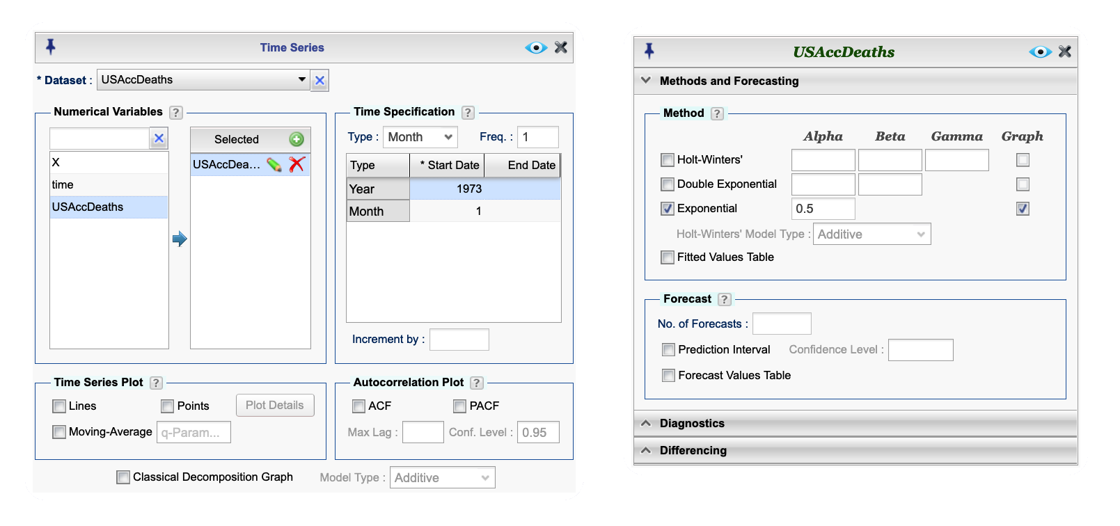
Figure 19.3: Time Series dialog for exponential smoothing plot.

19.4 Exponential Smoothing with Trend (Double-Exponential)

Instructions for exponential smoothing in Rguroo

1. Use a dataset in your Rguroo account or recreate the example below by importing the USAccDeaths dataset from the Rguroo dataset repository called R Datasets into your account.

Click here to see a portion of the dataset.

2. Open the Analytics toolbox on the left-hand side of the Rguroo window. Click on the Analysis dropdown menu and choose the Time Series function (see Figure 19.4) .

3. Select your dataset from the Dataset dropdown menu. In this example, we select the USAccDeaths dataset.

4. From the Numerical Variables section, select and drag the variable USAccDeaths to the Selected column.

5. (Optional) Under the Time Specification section, from the Type dropdown, select the time frequency of your data (yearly, quarterly, monthly, daily, hourly, by minute or seconds). The USAccDeaths data are monthly, so we select Month from the Type dropdown menu. Then set an appropriate start month and year for the data. The USAccDeaths data starts from January 1, 1973 so set Year to \(\tt{1973}\) and Month to \(\tt{1}\).

6. Click on the button to open the modeling dialog.

7. In the Methods and Forecasting dialog under the Method section, check Double Exponential and Graph.

8. In the text field to the right of Double Exponential, optionally enter an Alpha and/or a Beta value between 0 and 1. If a value is not specified, a default value will be chosen by Rguroo. We use a value of 0.5 for Alpha and 0.3 for Beta are used for this example.

9. Click the Preview icon to view the graph.

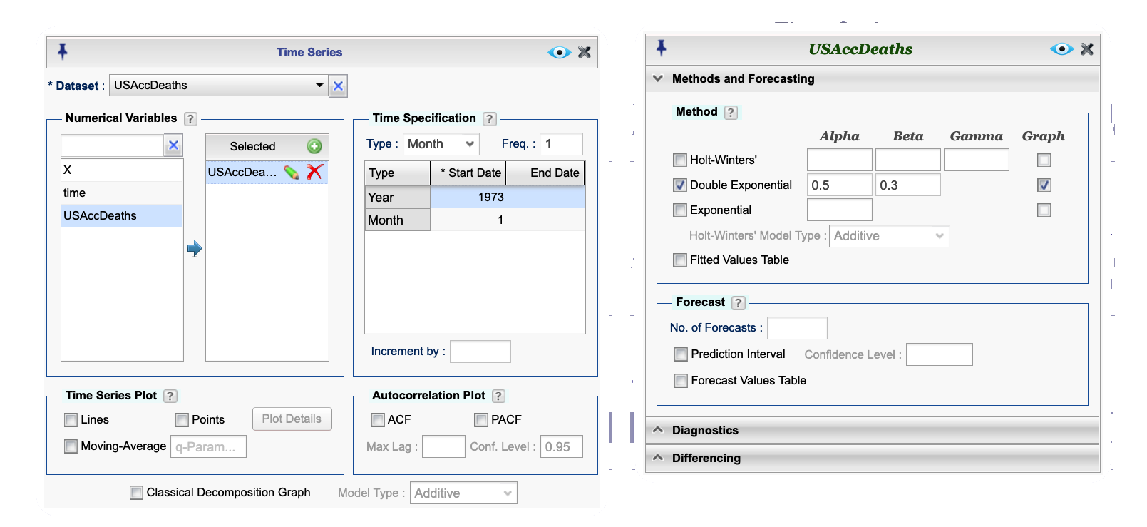
Figure 19.4: Time Series dialog for double exponential smoothing plot.

19.5 Additive and Multiplicative Seasonal Smoothing (The Holt-Winters Method)

Instructions for Holt-Winters in Rguroo

1. Use a dataset in your Rguroo account or recreate the example below by importing the AirPassengers dataset from the Rguroo dataset repository called R Datasets into your account.

Click here to see a portion of the dataset.

2. Open the Analytics toolbox on the left-hand side of the Rguroo window. Click on the Analysis dropdown menu and choose the Time Series function (see Figure 19.5) .

3. Select your dataset from the Dataset dropdown menu. In this example, we select the AirPassengers dataset.

4. From the Numerical Variables section, select and drag the variable AirPassengers to the Selected column.

5. Under the Time Specification section

• In the text field next to Freq., enter an integer value greater than or equal to 2 representing the number of observations per unit of time (4 for quarterly data, 12 for monthly data, etc.). A Freq. value of 12 is used for this example.
• (Optional) From the Type dropdown, select the time frequency of your data (yearly, quarterly, monthly, daily, hourly, by minute or seconds). The AirPassengers data are monthly, so we select Month from the Type dropdown menu. Then set an appropriate start month and year for the data. The AirPassengers data starts from January 1, 1949 so set Year to \(\tt{1949}\) and Month to \(\tt{1}\).

5. Click on the button to open the modeling dialog.

6. In the Methods and Forecasting dialog under the Method section, check Holt-Winters’ and select the Graph checkbox.

7. In the text field to the right of Double Exponential, optionally enter an Alpha, Beta, and/or Gamma value between 0 and 1. If a value is not specified, a default value will be chosen by Rguroo. In this example we use Rguroo’s default values.

8. In the dropdown menu labeled Holt-Winters’ Model Type select one of Additive or Multiplicative for the type of seasonal smoothing. We select Additive for this example.

9. Click the Preview icon to view the graph.

Time series plot of the AirPassengerData dataset.

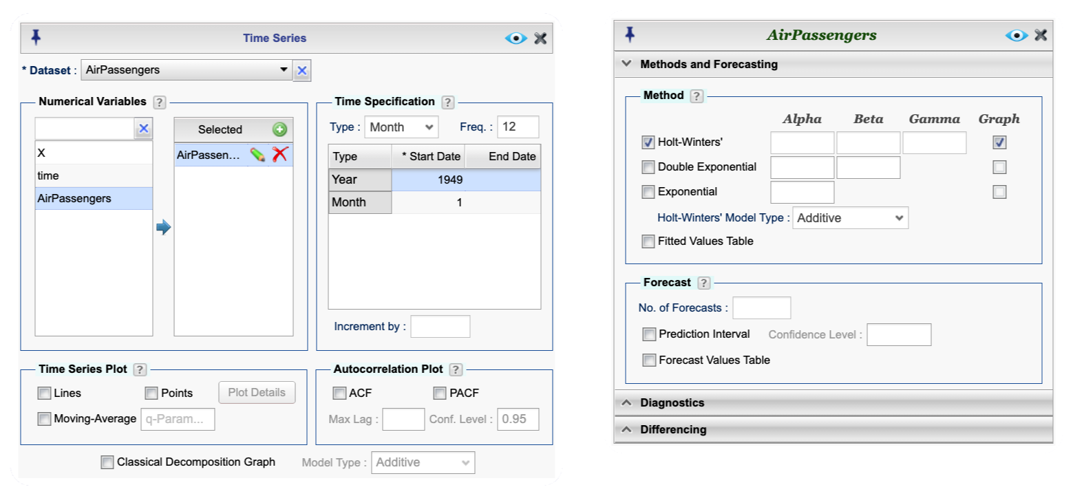
Figure 19.5: Time Series dialog for Holt-Winters plot.

19.6 Classical Decomposition Graph

Instructions for classical decomposition in Rguroo

1. Use a dataset in your Rguroo account or recreate the example below by importing the AirPassengers dataset from the Rguroo dataset repository called R Datasets into your account.

Click here to see a portion of the dataset.

2. Open the Analytics toolbox on the left-hand side of the Rguroo window. Click on the Analysis dropdown menu and choose the Time Series function (see Figure 19.6).

3. Select your dataset from the Dataset dropdown menu. In this example, we select the AirPassengers dataset.

4. From the Numerical Variables section, select and drag the variable AirPassengers to the Selected column.

5. Under the Time Specification section

• In the text field next to Freq., enter an integer value greater than or equal to 2 representing the number of observations per unit of time (4 for quarterly data, 12 for monthly data, etc.). A Freq. value of 12 is used for this example.
• (Optional) From the Type dropdown, select the time frequency of your data (yearly, quarterly, monthly, daily, hourly, by minute or seconds). The AirPassengers data are monthly, so we select Month from the Type dropdown menu. Then set an appropriate start month and year for the data. The AirPassengers data starts from January 1, 1949 so set Year to \(\tt{1949}\) and Month to \(\tt{1}\).

6. At the bottom of the dialog, select Classical Decomposition Graph.

7. From the Model Type dropdown menu to the right of the Classical Decomposition Graph checkbox, select one of Additive or Multiplicative.

8. Click the Preview icon to view the graph.

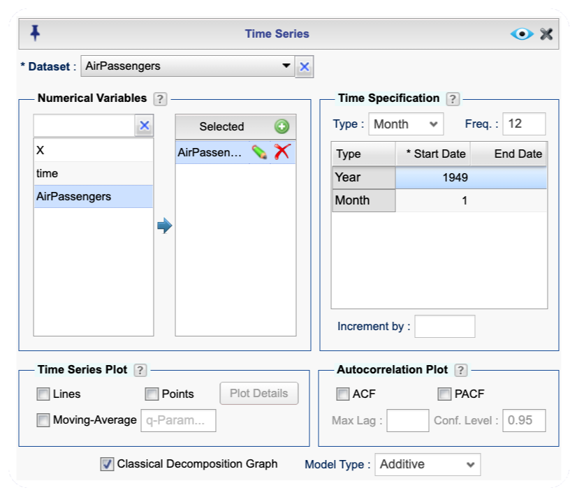
Figure 19.6: Time Series dialog for decomposition graph.

19.7 Fitted Values and Residuals

Instructions to obtain fitted values and residuals in Rguroo

1. Use a dataset in your Rguroo account or recreate the example below by importing the USAccDeaths dataset from the Rguroo dataset repository called R Datasets into your account.

Click here to see a portion of the dataset.

2. Open the Analytics toolbox on the left-hand side of the Rguroo window. Click on the Analysis dropdown menu and choose the Time Series function (see Figure 19.7) .

3. Select your dataset from the Dataset dropdown menu. In this example, we select the USAccDeaths dataset.

4. From the Numerical Variables section, select and drag the variable USAccDeaths to the Selected column.

5. (Optional) Under the Time Specification section, from the Type dropdown, select the time frequency of your data (yearly, quarterly, monthly, daily, hourly, by minute or seconds). The USAccDeaths data are monthly, so we select Month from the Type dropdown menu. Then set an appropriate start month and year for the data. The USAccDeaths data starts from January 1, 1973 so set Year to \(\tt{1973}\) and Month to \(\tt{1}\).

6. Click on the button to open the modeling dialog.

7. In the Methods and Forecasting dialog under the Method section

• Check the modeling method(s) you would like to use (Exponential, Double Exponential, and/or Holt-Winters). Alpha, Beta, and Gamma parameters may be optionally specified in the text fields. For this example, we choose the (Exponential and Double Exponential methods with default values of Alpha and Beta.
• Select the Fitted Values Table checkbox.

8. Click the Preview icon to view the graph.

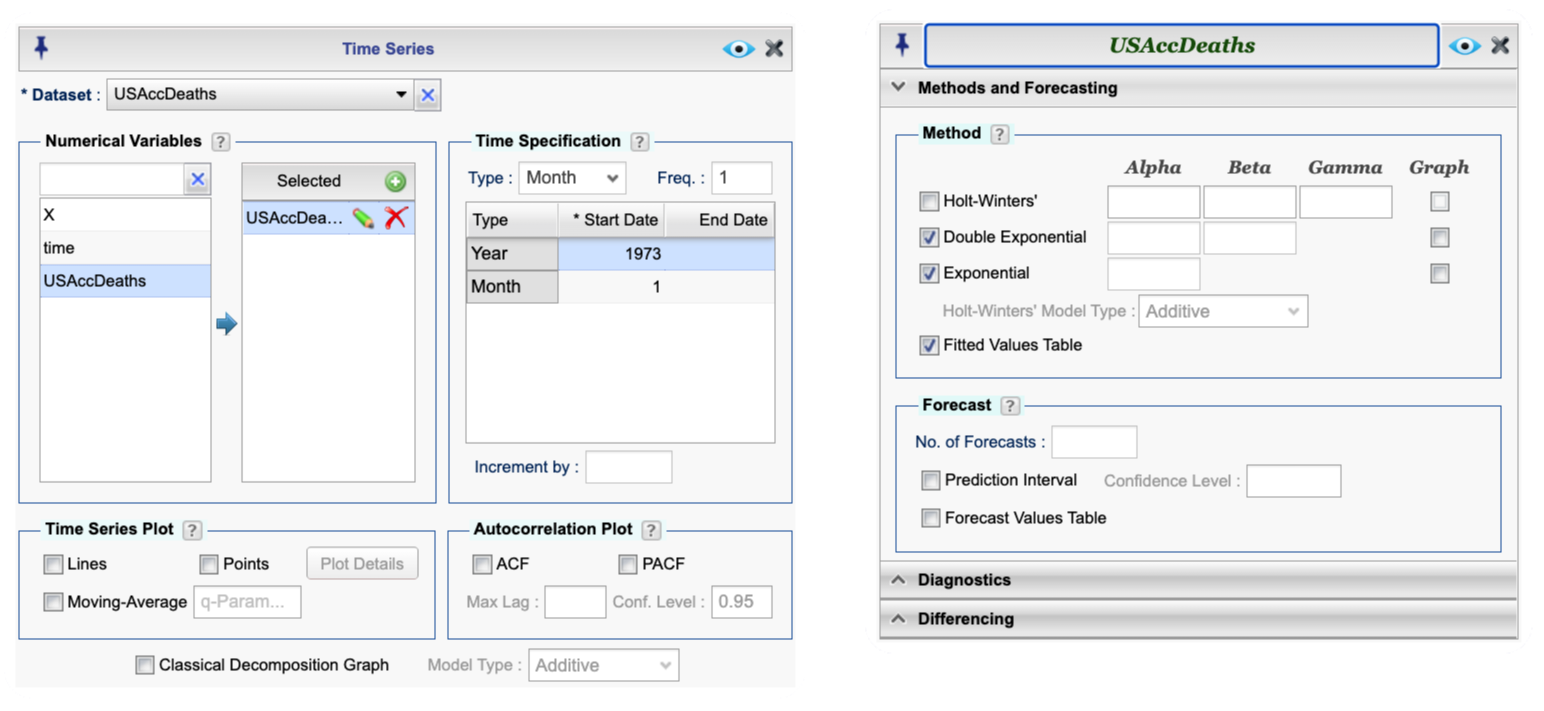
Figure 19.7: Time Series dialog for forecasting error.