14 Logistic Regression

In this section we explain how to use Rguroo to fit a logistic regression model to data including various diagnostics and prediction assessment tools.

You can access Rguroo’s Logistic Regression function (tab) under the Analytics toolbox. The Logistic Regression function has two options of Binary Response Data or Grouped Data. With the Binary Response Data option you specify a single variable that consists of events (successes) and nonevents (failures); this can be done in various ways, as we explain in Section 14.1. Using the Grouped Data option, you specify two variables that include two of the following three pieces of information for each group: the number of events, the number of nonevents, or the total number of observations (trials); this is explained in Section 14.2.

14.1 Specifying Events and non-Events with Binary Response Data

To perform logistic regression with binary response data, go to the Analytics toolbox and use the clickstream Logistic Regression —> Binary Response Data. This opens the Logistic Regression dialog for binary data, shown in Figure 14.1. You can open and close this dialog by clicking on the Basics Button button.

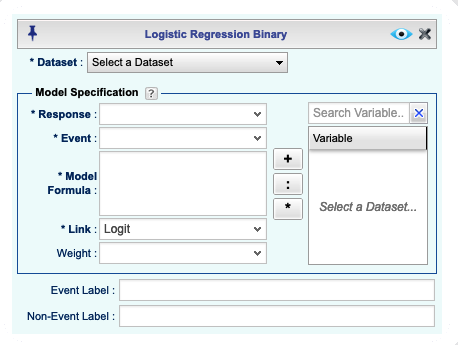
Figure 14.1: Logistic Regression basics Dialog for Binary Data

In the Logistic Regression dialog, you can specify the response and the event in one of the following ways:

Selecting a Categorical Variable: If you select a categorical (factor) variable from the Response dropdown as your response variables, then the levels of the selected categorical variable will appear in the Event dropdown. From this dropdown, you must choose a level that corresponds to the event (success). By default, the label for the event is the default label for the selected level. However, you can enter a different label for the event in the Event Label textbox. Similarly, you enter a label for the non-event (failure) in the Non-Event Label textbox.
Selecting a Numerical Variable: If you select a numerical variable from the Response dropdown, you must enter a specific value of the selected variable that represents the event (success). Non-events (failures) will be all values from the variable not equal to that specified in the Event textbox. Typically, the numerical variables that indicate the event and non-event consist of 0 and 1, but Rguroo does not restrict the values to be 0 or 1. You can enter a label for the event in the Event Label textbox and a label for the non-event in the Non-Event Label textbox.
Specifying an R Logical Expression: You can type an R logical expression in the Response textbox. The expression must evaluate to a logical vector of the same length as the number of observations in the dataset with values TRUE (1) and FALSE (0). After typing the expression, the Event dropdown will consist of two elements, 0 (FALSE) and 1 (TRUE), one of which you must select to represent the event. Typically, the logical expression is written so that the value of TRUE (1) represents the event. You can enter a label for the event in the Event Label textbox and a label for the non-event in the Non-Event Label textbox.

14.2 Specifying Events and Non-Events for Grouped Data (Event-Trial Data)

To perform logistic regression with grouped data, go to the Analytics toolbox and use the click stream Logistic Regression —> Grouped Data. This opens the *Logistic Regression Grouped Data** dialog for grouped data, shown in Figure 14.2. You can open and close this dialog by clicking on the Basics Button button.

In this dialog, there are three dropdowns labeled Trials, Event, Non-Event. These dropdowns include names of all numerical variables in your selected dataset. You must select two variables from two of the dropdowns indicating one of the pairs (Trial, Event), (Trial, Non-Event), or (Event, Non-Event). The trial dropdown should include a variable that represents the total number of observations (trials) for each group. The event and non-event dropdowns should include variables that represent the number of events and nonevents for each group. Note that the selected variables for events and non-events must be non-negative integers, and the values for the trial must be positive integers.

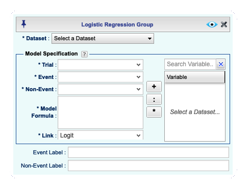
Figure 14.2: Logistic Regression basics Dialog for Grouped Data

14.3 Specifying the Model Formula

You can specify your predictors and the model formula in the textbox labeled Model Formula in the Logistic Regression dialog; see Figure 14.1. Predictors must be separated by a “+” sign. To get a model without an intercept, add a “-1” to your formula. You can add interactions using asterisk “*” or colon “:”. For example, the formula x1 + x2 + x1:x2 includes the main effects of x1 and x2 and the interaction between x1 and x2. For details on specifying models see the following R documentation.

14.4 Specifying the Link Function and Weights

You can specify the link function and the weights in the Logistic Regression dialog.

The Link dropdown lets you choose between the logit, probit, and complementary log-log link functions.

If cases are to be weighted, the Weight dropdown allows you to choose a numerical variable for your weights. This variable must contain non-negative values. If you select a variable from the Weight dropdown, the weights will be used in the fitting process. If you do not choose a variable, the weights will be set to 1 for all cases. Cases with a weight of zero will not be used in fitting the model.

The Weight dropdown is not available for grouped data.

14.5 Estimates and Diagnostics Output

The logistic regression output reports includes a set of default and optional components that you can select or deselect. To select or deselect specific estimates and diagnostics components, click the Details button button in the Logistic Regression tab. This opens the Logistic Regression Details window. From there, select Estimates and Diagnostics to open the Estimates and Diagnostics dialog shown in Figure 14.3. The components of default output are shown in the Selected column in the figure, and additional outputs are shown in the column labeled Options. You can select and deselect components by moving them between the two columns using the left and right arrows or by drag-and-drop between the two columns.

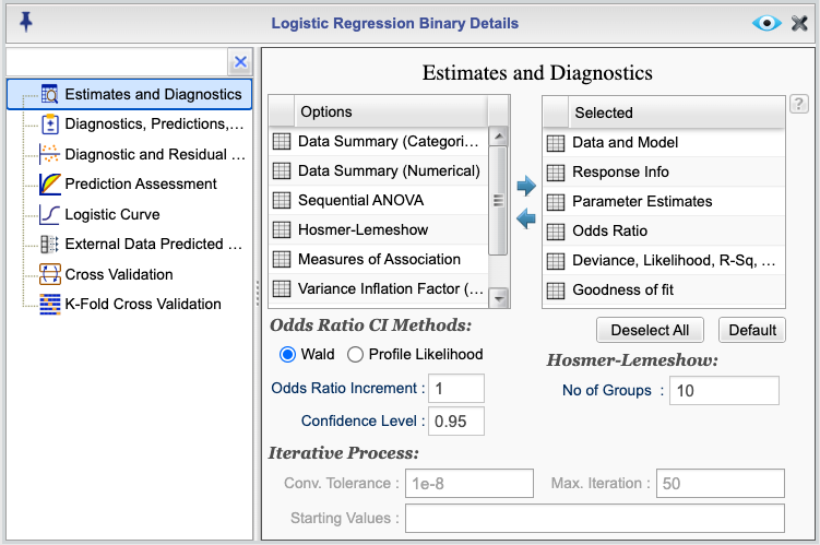
Figure 14.3: Logistic Regression Estimates and Diagnostics Dialog

The following is a description of the content of the tables that are generated by selections made in the Estimates and Diagnostics dialog:

Data and Model: This table provides a summary of the data, the method (link) used, and the model specified.
Response Info: This table provides information about the number of events and nonevents in the data, and their labels.
Parameter Estimates: This table provides the estimated coefficients, standard errors, z-values, and p-values for the model coefficients.
Odds Ratios: This table provides the odds ratios and their confidence intervals. Two methods of Wald and Profile Likelihood are available. The default method is Wald. You can select the Profile Likelihood method by choosing the Profile Likelihood option shown in the dialog.
Deviance, Likelihood, R-squared, AIC, BIC: This table a few measures of model fit including the deviance, null deviance (deviance for the intercept-only model), MSE (Brier Score), R-squared, adjusted R-squared, the Akaike Information Criterion (AIC), and the Bayesian Information Criterion (BIC).
Goodness-of-Fit: This table provides the results of Deviance, Pearson, and the Hosmer-Lemeshow goodness-of-fit tests. The default number of groups for the Hosmer-Lemeshow test is 10. In the Estimates and Diagnostics dialog, you can change this number by entering a different value in the Number of Groups textbox.
Data Summary (Categorical): This table provides the number of levels and the levels of the categorical variables in the model if any.
Data Summary (Numerical): This table outputs the number of observations for each numerical variable in the model, the five-number summary, and the mean.
Sequential ANOVA: This table provides the sequential analysis of variance as variables are entered into the model in the order specified in the model formula.
Hosmer-Lemeshow: This table provides the event probability intervals and the observed and expected frequencies for events and non-events for each probability interval used in computing the Hosmer-Lemeshow test. Note that the number of groups for this test has a default of 10 and can be set in the No of Groups textbox in the Estimates and Diagnostics dialog.
Measures of Association: This table includes the following measures of association: Concordant, Discordant, Somers’ D, Goodman-Kruskal Gamma, and Kendall’s Tau-a.
Variance Inflation Factor (VIF): This table provides generalized variance inflation factors (GVIF) and a scaled generalized inflation factor with the corresponding degrees of freedom.
Covariance of Parameter Estimates: This table provides the covariance matrix of the parameter estimates.
Iterative Process: This table provides information such as convergence status, number of iterations, convergence tolerance used, the maximum number of iterations allowed, and the deviance and the likelihood value at the point when the iterative process has stopped.

14.5.1 Odds Ratio, Hosmer-Lemeshow, and Iterative Process Options

Within the Estimates and Diagnostics dialog, you can control the following parameters related to the iterative process: - Conv Tolerance: The convergence tolerance is the criterion used to determine when the iterative process has converged. The default value is 1e-8. You can change this value by entering a different value in the Conv. Tolerance textbox. - Max Iterations: The maximum number of iterations allowed for the iterative process. The default value is 50. You can change this value by entering a different value in the Max Iterations textbox. - Starting Values: The starting values for the parameter estimates. The default is determined internally by R. However, to overwrite the default, you must provide a starting value for each parameter in the model ordered by the order of the predictors in the model formula. Values should be comma-separated. Generally, the first estimate is for the intercept (if the model includes an intercept); for each numerical predictor, you would need one estimate, and for each categorical predictor, you need one estimate for each level of the predictor, except for the reference level.

14.6 Diagnostics, Predictions, and Residuals Table

You can obtain predictions, residuals, and diagnostic indices for each observation by clicking the Details button button in the Logistic Regression tab and selecting Diagnostics, Predictions, Residuals from the list provided in the Logistic Regression Details window. This opens the Diagnostics, Predictions, Residuals dialog shown in Figure 14.4.

In this dialog, select the checkbox Show Table. This generates a table of diagnostics, predictions, and residuals for each observation. You can specify a confidence level for prediction intervals; the default is 0.95. You can also optionally select a variable from the ID Variable dropdown to identify each case in the output table.

The first column of the table will be the case numbers. If you select an ID variable, the second column will be the values of the ID variable. The remaining columns will be determined by the quantities in the Selected column. The default values are those shown in the Selected column in Figure 14.4, and additional options are shown in the column labeled Options. You can select and deselect components by moving them between the two columns using the left and right arrows or by drag-and-drop between the two columns.

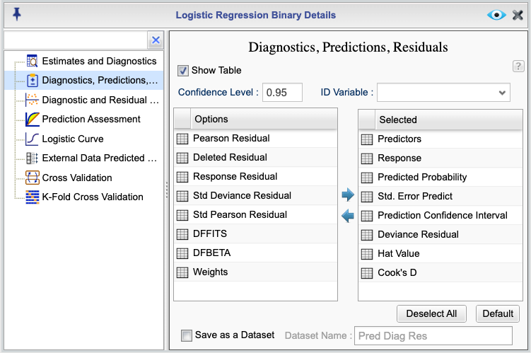
Logistic Regression Diagnostics, Predictions, and Residuals Dialog

Figure 14.4: Diagnostics, Predictions, and Residuals Dialog

The following is a description of each of the options in the Diagnostics, Predictions, Residuals dialog:

Predictors: The values of the predictors used in the model.
Response: The values of the response variable.
Predicted Probability: The predicted probability of the event for each case based on the fitted model.
Std. Error Predict: The standard error of the predicted probabilities.
Prediction Confidence Interval: The lower and upper bounds of the 95% confidence interval for the predicted probabilities.
Deviance Residual: The deviance residuals.
Hat Value: The hat values, indicating leverage.
Cook’s D: The Cook’s distance.
Pearson Residual: The Pearson residuals.
Deleted Residual: The deleted residuals.
Response Residual: The response residuals.
Std Deviance Residual: The standardized deviance residuals.
Std Pears Residual: The standardized Pearson residuals.
DFFITS: The DFFITS values.
DFBETAS: The DFBETAS values.
Weights: The weights used in the fitting process, if weights are used.

14.7 Diagnostic and Residual Plots

To access diagnostic plots, click the Details button button in the Logistic Regression tab. This will open the Logistic Regression Details window. From there, select the Diagnostic and Residual Plots option to view the Diagnostics and Residual Plots dialog, shown in Figure 14.5. In this dialog, choose Show Plots to generate your desired diagnostic plots. The default diagnostic plots are shown in the Selected column in the figure, and additional options are presented in the Options column. You can select or deselect components by moving them between the two columns using the left and right arrows or by using drag-and-drop.

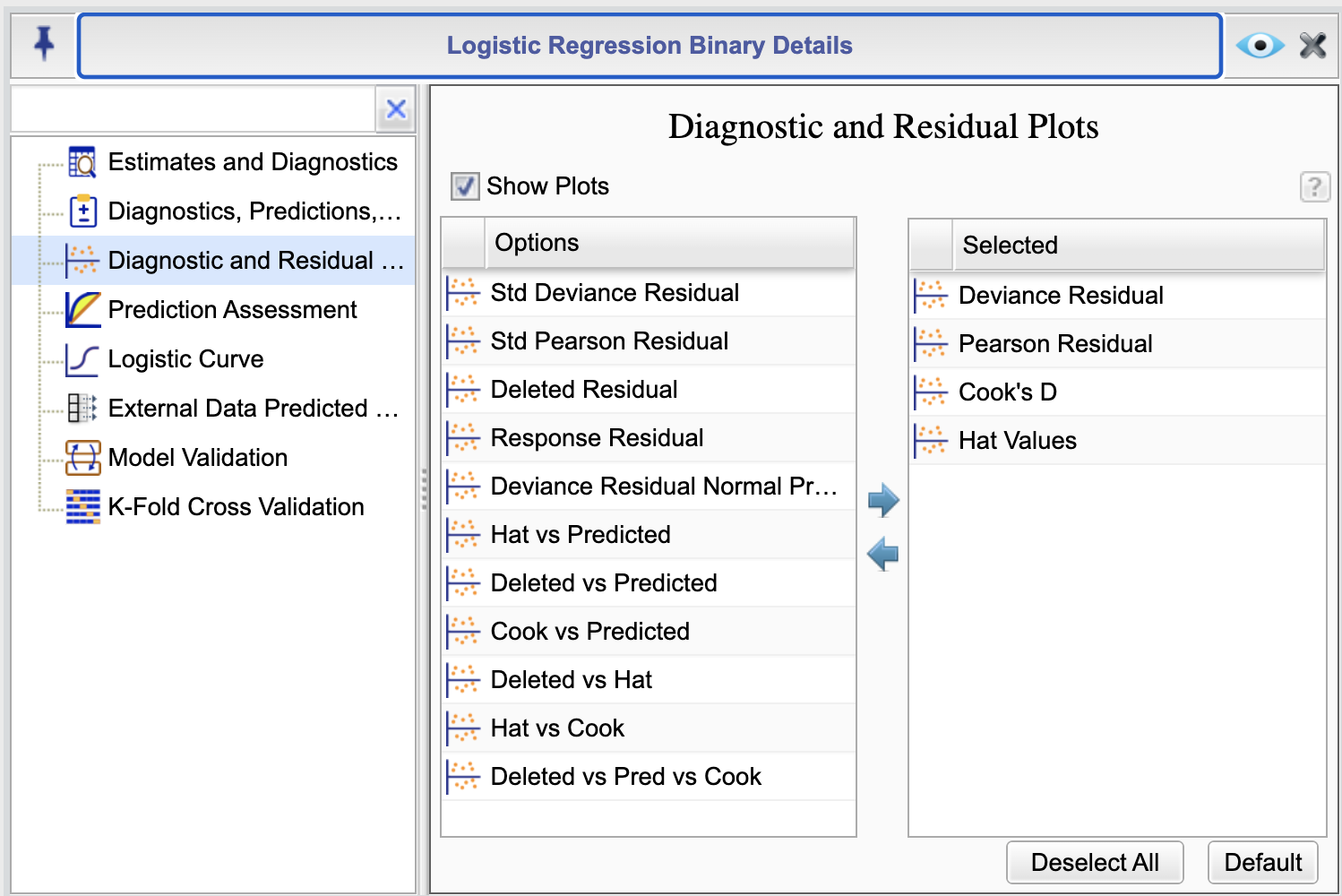
Logistic Regression Diagnostic and Residual Plots Dialog

Figure 14.5: Diagnostics and Residual Plots Dialog

The following is a description of each option in the Diagnostic and Residual Plots dialog. All scatterplots identify a few outlier cases by their case numbers:

Deviance Residual: This option plots a histogram of the deviance residuals and a scatterplot of the deviance residuals against the case numbers.
Pearson Residual: This option plots a histogram of the Pearson residuals and a scatterplot of the Pearson residuals against the case numbers.
Cook’s Distance: This option plots Cook’s distance against the case numbers.
Hat Values: This option plots the hat values against the case numbers.
Std Deviance Residual: This option plots a histogram of the standardized deviance residuals and a scatterplot of the standardized deviance residuals against the case numbers.
Std Pearson Residual: This option plots a histogram of the standardized Pearson residuals and a scatterplot of the standardized Pearson residuals against the case numbers.
Response Residual: This option plots a histogram of the response residuals and a scatterplot of the response residuals against the case numbers.
Deleted vs Pred vs Cook: This option plots a bubble plot that includes a plot of the deleted residuals against the predicted probabilities. The bubble size is proportional to Cook’s distance.
Hat vs Predicted: This option plots the hat values against the predicted probabilities.
Deleted vs Predicted: This option plots deleted residuals against the predicted probabilities.
Cook vs Predicted: This option plots Cook’s distance against the predicted probabilities.
Deleted vs Hat: This option plots deleted residuals against the hat values.
Cook vs Hat: This option plots Cook’s distance against the hat values.

14.8 Prediction Assessment

Rguroo provides various options for assessing model predictions. To access these options, click the Details button button in the Logistic Regression tab. This will open the Logistic Regression Details window. From there, select the Prediction Assessment option to view the Prediction Assessment dialog, shown in Figure 14.6. In this dialog, select the checkbox Perform Assessment to enable assessment options. This dialog consists of two tabs: Accuracy, shown in Figure 14.6, and ROC Analysis, shown in Figure 14.7. You can select or deseclt options by checking or unchecking boxes.

Logistic Regression Prediction Assessment Dialog

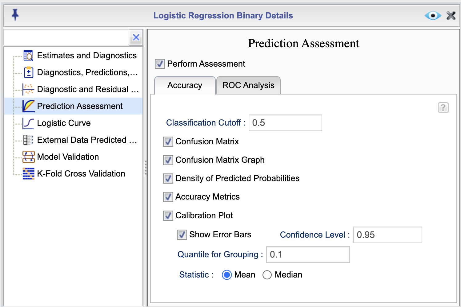
Figure 14.6: Prediction Assessment Dialog

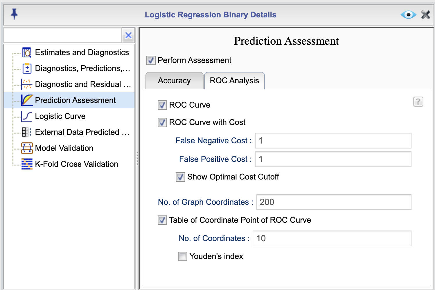
Figure 14.7: Prediction Assessment Dialog

To obtain prediction assessments metrics, specify a value in the Classification Cutoff textbox in teh Accuracy tab. This value is used to classify the predicted probabilities into events and non-events. The default value is 0.5. You can change this value by entering a different value in the textbox.

The following is a description of each option in the Prediction Assessment dialog Accuracy tab:

Confusion Matrix: This option generates a confusion matrix that shows the number of true positives, true negatives, false positives, and false negatives.
Confusion Matrix Graph (not available for the Grouped Data option): This is a graphical display of the confusion matrix. It displays a graph of predicted probabilities (scores) against observed responses; observed responses are jittered to avoid as much overlap as possible.
Density of Predicted Probabilities (not available for the Grouped Data option): This option generates a density plot of the predicted probabilities for events and non-events.
Accuracy Metrics: This option provides the following accuracy metrics: True Positive, True Negative, False Positive, False Negative, Sensitivity, Specificity, Precision, Negative Predictive Value, False Positive Rate, False Negative Rate, False Discovery Rate, False Omission Rate, Prevalence, Accuracy, and F1 Score.
Calibration Plot: This option generates a calibration plot that shows the observed responses against the predicted probabilities. The plot is divided into groups based on the quantiles of the predicted probabilities. YOu can specify the your desired quantile in the textbox Quantile for Grouping; the default value is 0.1 that creates approximately 10 groups. The observed responses are averaged for each group and plotted against the average predicted probabilities. You can also add error (confidence) bars to the plot by selecting the Show Error Bar option, and you can set a confidence level for the error bars by entering a value in the Confidence Level textbox. The default value is 0.95.

The following is a description of each option in the Prediction Assessment dialog ROC Analysis tab:

ROC Curve: This option generates a receiver operating characteristic (ROC) curve. The ROC curve is a plot of the true positive rate (sensitivity) against the false positive rate (1-specificity) for the specified classification cutoff. The area under the ROC curve (AUC) is also provided. The following three options are available for the ROC curve:
- ROC Curve with Cost: This option provides the ROC curve and an additional graph showing the cost. The cost is determined based on the values that you input in the textboxes False Negative Cost and False Positive Cost. The default for both cost values is set to 1.
- Show Optimal Cost Cutoff: By selecting this option, when the option ROC Curve with Cost is selected, you will get an optimal cutoff value that minimizes the cost.
- No. of Graph Coordinates: This option specifies the number of points used to plot the ROC curve. The default value is 200. You can change this value by entering a different value in the No. of Graph Coordinates textbox.
- Table of ROC Coordinates: This option provides a table of the coordinates of the ROC curve. You can specify the number of coordinates to be printed in the textbox No. of Coordinates The table includes the cutoff, Sensitivity (true positive rate), 1 - Specificity (false positive rate), Miss Rate (false negative rate), cost (if cost plot selected), and the Yoden’s index (if selected).

14.9 Graph of Logistic and Other Link functions for single and multiple predictors

You can use Rguroo to plot a curve of the logistic function or other link functions in your model if you have at least one numerical predictor. If your model has multiple predictors, you can choose the numerical predictor for the horizontal axis and set the rest of the predictors to specific fixed values. You also have the option to plot logistic curves for all levels of a categorical variable. Additionally, you can optionally plot confidence curves for the logistic curve and plot the observed responses.

To access the logistic curve function, click the Details button button in the Logistic Regression tab. This will open the Logistic Regression Details window. From there, select the Logistic Curve option to view the Logistic Curve dialog, shown in Figure 14.8.

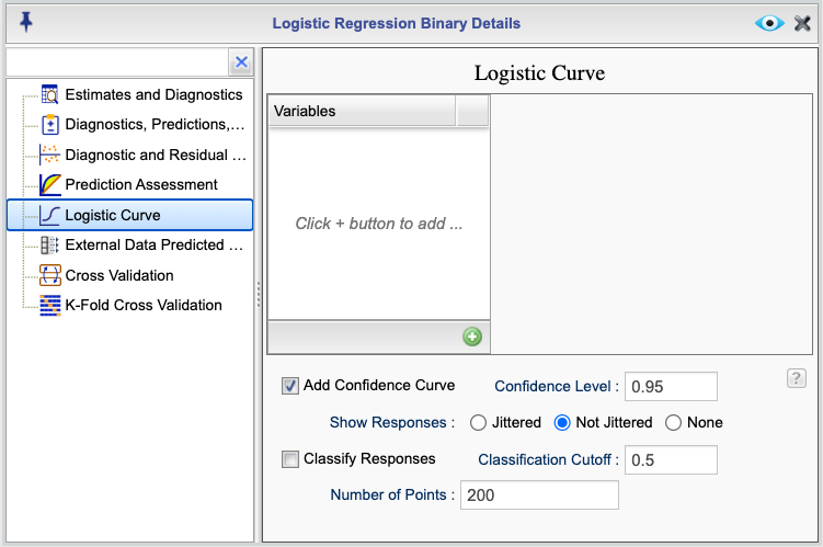
Figure 14.8: Logistic Curve Dialog

The Logistic Curve dialog allows you to create multiple graphs. To specify a graph, begin by clicking on the Add button button. This will add a dropdown menu consisting of the numerical predictors to the column labeled Variables. Select a numerical predictor from the dropdown menu. Once you select a numerical variable, all other predictor variables will appear in the adjacent column, with numerical predictors, by default, set to their mean value (rounded) and categorical predictors set to their reference level.

You can fix the values of numerical predictors by typing a value into the provided textboxes. For categorical predictors, you can select a level from the dropdown menu shown for them. There is an option to plot the logistic curve for all levels of a categorical variable by selecting the All Levels option from the dropdown. Note that you can use the All Levels option for only one categorical variable.

The following are additional options available for your graph:

Confidence Curve: This option plots the confidence curve for the logistic curve. You can specify the confidence level by entering a value in the Confidence Level textbox. The default value is 0.95.
Show Responses: There are three options of Jittered, Not Jittered, and None. The option Jittered jitters the observed responses to avoid overlap as much as possible. The option Not Jittered plots the observed responses without jittering. The option None suppresses the observed responses.
Classify Responses: This option annotates the observed responses on the graph based on their classification of true Positive (TP), true negative (TN), false positive (FP), and false negative (FN). This option is especially useful if you plot responses using the jittered option.
Classification Cutoff: This option specifies the classification cutoff value. The default value is 0.5. You can change this value by entering a different value in the Classification Cutoff textbox.
Number of points: This option specifies the number of points used to divide the values in the horizontal axis. The default value is 200. You can change this value by entering a different value in the Number of Points textbox.

14.10 External Data Prediction Propbabilities

You can use the logistic regression function in Rguroo to obtain predicted probabilities (probability of being an event) for specified predictor values not used in fitting the model, referred to as external data. To access this option, click the Details button button in the Logistic Regression tab. This will open the Logistic Regression Details window. From there, select the External Data Prediction Probabilities option to view its dialog. Figure 14.9 shows an example of the Prediction Probabilities dialog for the example that we will show in Section 14.12.

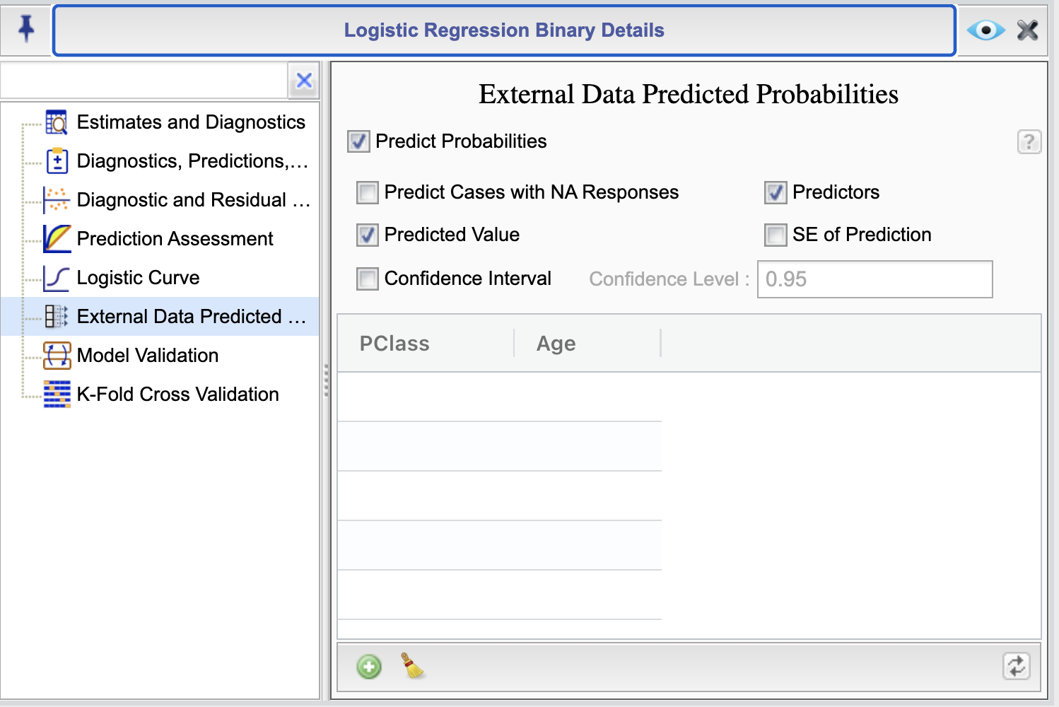
Figure 14.9: External Data Prediction Probabilities Dialog

The External Data Prediction Probabilities dialog allows you to specify the values of the predictors for which you want to obtain predicted probabilities. To begin, you need to select the checkbox Predict Probabilities To specify the values of the predictors, this dialog consists of a table with columns indicating the predictor variables. You can type in numerical values in the numerical variable columns and select levels for categorical variables from the dropdown menus that appear in categorical variable columns. You can add rows to the table by clicking the Add button button, as needed. Note that if you change predictors in your model, then you should use the refresh button , shown at the bottom of the dialog, to get the new predictors in the edit area. The clear all button is used to clear all the values in the table.

Alternatively, or additionally, you can add rows to the dataset used to fit the model and set the response variable to NA for the cases you want to predict. To obtain the predicted probabilities for these cases in the output report, select the checkbox Predict Cases with NA Responses.

By default the Predictors and Predicted Value checkboxes are selected. With these options the table of predictions will include the values of predictors and their corresponding predicted probabilities. By selecting the checkboxes SE of Prediction and Confidence Interval, you can include the standard error of the predicted probabilities and a confidence interval for the predicted probabilities, respectively. You can specify the confidence level for the confidence interval by entering a value in the Confidence Level textbox. The default value is 0.95.

14.11 Model Validation

You can use Rguroo’s Model Validation function to assess your model performance. To access this option, click the Details button button in the Logistic Regression tab. This will open the Logistic Regression Details window. From there, select the Model Validation option to view the Model Validation dialog, shown in Figure 14.10.

To begin model validating, select the checkbox Start Validation. Note that you cannot apply the function K-Fold and Model Validation at the same time.

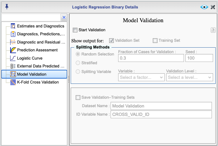
Figure 14.10: Cross-Validation Dialog

14.11.1 Choice of output

When performing model validation, there are two options for requesting output: Validation Set and Training Set. By default, By default, Rguroo will display all of your choices in the Prediction and Assessment dialog (see Section 14.8) for the validation set. However, if you check the Training Set checkbox in the Model Validation dialog you also get the requested Prediction and Assessment output for the training set.

Selected outputs from the following dialogs will be based on the training set: - Estimates and Diagnostics: See Section 14.5 for the output choices.

Diagnostics, Predictions, and Residuals: See Section 14.6 for the output choices.
Diagnostic and Residual Plots: See Section 14.7 for the output choices.
Logistic Curve: See Section 14.9 the output choices.

14.11.2 Methods for splitting data

The Model Validation dialog provides three methods for splitting the data into training and validation sets:

Random: This method randomly splits the data into training and validation sets; select the option Random Selection for this choice. You can specify the proportion of the data to be used for the validation set by entering a value in the Fraction of Cases for Validation textbox. The default value is 0.3.
Stratified: This method splits the data into training and validation sets while maintaining the proportion of events and nonevents in each set; select the option Stratified for this choice. You can specify the proportion of the data to be used for the validation set by entering a value in the Fraction of Cases for Validation textbox. The default value is 0.3. As an example, if there are 100 cases, of which 43 are events and 57 are non-events, and the selected fraction for the validation set is 0.3, then round(0.3 * 43) = 13 cases will be selected randomly from the 43 events and round(0.3 * 57) = 17 cases will be randomly selected from the 57 non-event cases.
Splitting Variable: This method splits the data into training and validation sets based on the values of an ID variable; select the option Splitting Variable for this choice. You can specify the ID variable by selecting a variable from the corresponding Variable dropdown that includes names of all categorical variables in the dataset. Once you select an ID variable, then you need to choose a level from the Level dropdown. The cases corresponding to the selecetd level will be used for the validation set and all other cases will be used for the training case. If the ID variable of your choice is numerical, you can change its type to categorical in Rguroo’s Dataset Editor (see Section 2.3.5). .

14.11.3 Saving Validation and Training Sets

You can save the validation and training sets by selecting the Save Validation – Training Sets checkbox. You need to specify a dataset name in the Dataset Name textbox and an ID variable name in the ID Variable Name textbox. Once you click the preview button, a dataset with the name that you specify will be created that includes all the variables used in the model with an ID variable column appended that identifies the cases in the validation and training sets. The saved dataset will be available under the Data toolbox.

14.12 An Example of Logistic Regression with Binary Data

To illustrate how to use some of Rguroo’s logistic regression options and review output reports, we use the Titanic1 dataset available in the Rguroo Users Guide dataset repository. This dataset contains the names of the passengers (Name) in the Titanic, the passenger class (PClass), the age of each passenger (Age), their gender (Sex), and whether they survived or not (Survived). The Survived variable is binary, where 1 indicating that the passenger survived and 0 indicating that the passenger did not survive.

We begin by modeling the probability of survival as a function of age and the passenger class.

14.12.1 Fitting the basic model

Recreate the example below by importing the Titanic1 dataset from the Rguroo Users Guide dataset repository into your account.

Click here to see a portion of the dataset.

Screenshot of the first 5 rows of the Titanic1 dataset.

On the left-hand side of the Rguroo window, open the Analytics toolbox. Use the Analysis dropdown menu and choose Logistic Regression —> Binary Data. The Logistic Regression Basics dialog will appear (see Figure 14.11).
Select a Dataset; for this example, the Titanic1 dataset.
In the Model Specification section, complete the following:
- Select your response variable from the Response dropdown; in this example, the variable Survived.
- Specify the value indicating the Event in the response variable; in this example, we type the value 1. See Section 14.1 for various options for specifying events.
- In the Model Formula textbox, specify the predictors. Predictors must be separated by a + sign. To get a model without an intercept, add -1 to your formula. See R documentation for details on how to specify models with interactions using “*” and “:”. For this example, we use Age + PClass.
- From the Link dropdown, select the link function. The default is the logistic link function.
In the Event Label textbox, type a label for the event. The default is the value specified for the “Event.” In this example, we use “Survived.”
In the Non-Event Label textbox, type a label for non-event(s). The default is the value specified for the “Event” with a “Not” added before it. In this example we use “Died.”
(Optional) Click the to add or modify output.
Click the Preview icon to view the result.

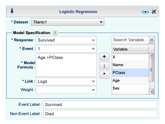
Figure 14.11: Logistic Regression Basics dialog

The Rguroo output is shown above. The output includes the following sections:

Data, Method, and Model, including the number of observed and missing data
Response Information, including the number of events and non-events
Parameter Estimates, including the estimated coefficients, standard errors, z-values, and p-values
Odds Ratios, including the odds ratios and their confidence intervals
Measures of Model Fit, including Deviance, Log-Likelihood, MSE, R-Squared, AIC, and BIC
Goodness of Fit Test, including Deviance, Pearson, and Hosmer-Lemeshow tests
Confusion Matrix, including True Positive, True Negative, False Positive, and False Negative counts and percentages.
Confusion Matrix Graph, including a graphical display of the confusion matrix.
Density of Predicted Probabilities, including density plots of the predicted probabilities for events and non-events.
ROC Plot and Cost Function Plot, including the ROC curve and the cost function plot, including the area under the curve (AUC) and optimal classification cutoff.

The output can be modified and expanded by selecting the Details button button in the Logistic Regression tab. This will open the Logistic Regression Details window, where you can select additional output options and set your desired parameters such as classification cutoffs and confidence levels.

14.12.2 Obtaining logistic curve graphs

Figure 14.12 shows the Rguroo dialog for obtaining logistic curve graphs for the example given in Section 14.12.1. In general, you can click the green plus sign button to add a dropdown in the Variables column. Each dropdown includes all numerical predictors in the model which you can select for the horizontal axis of the logistic curve. In our example, the only predictor is Age. The other predictors are set to their mean value for numerical predictors and to their reference level for categorical predictors. You can fix the values of numerical predictors by typing a value into the provided textboxes. For categorical predictors, you can select a level from the dropdown menu shown for them. You can plot logistic curves for all levels of a categorical variable by selecting the All Levels option from the dropdown. Note that you can use the All Levels option for only one categorical variable.

In this example, we are drawing two logistic curve graphs for the variable Age. In one case, we set the value of the variable PClass to 1, which is the reference level for the variable, and in another case we set the variable PClass to “All Levels” to see the logistic curve for all levels simultaneously. The results are shown in Figures 14.13 and 14.14, respectively.

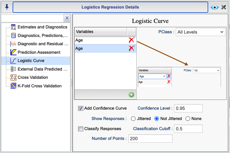
Figure 14.12: Logistic Curve Dialog

Figure 14.13: Logistic Curve for Age and First Class Passengers

Figure 14.14: Logistic Curve for Age and All Levels of PClass

14.12.3 Predicting success probabilities for external (new) data

You can predict probability of success (event) for new data by selecting the External Data Predicted Probabilities from the Logistic Regression Details , shown in Figure 14.15. In this example we are predicting probability of survival for those age 32 and 60 and being in first, second, or third passenger class. The predicted values are shown in Figure 14.16.

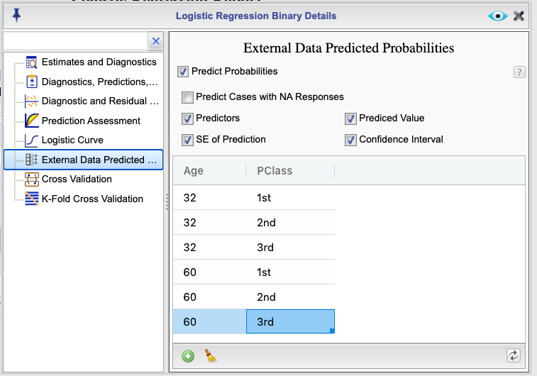
Figure 14.15: Dialog for predicting external data probabilities

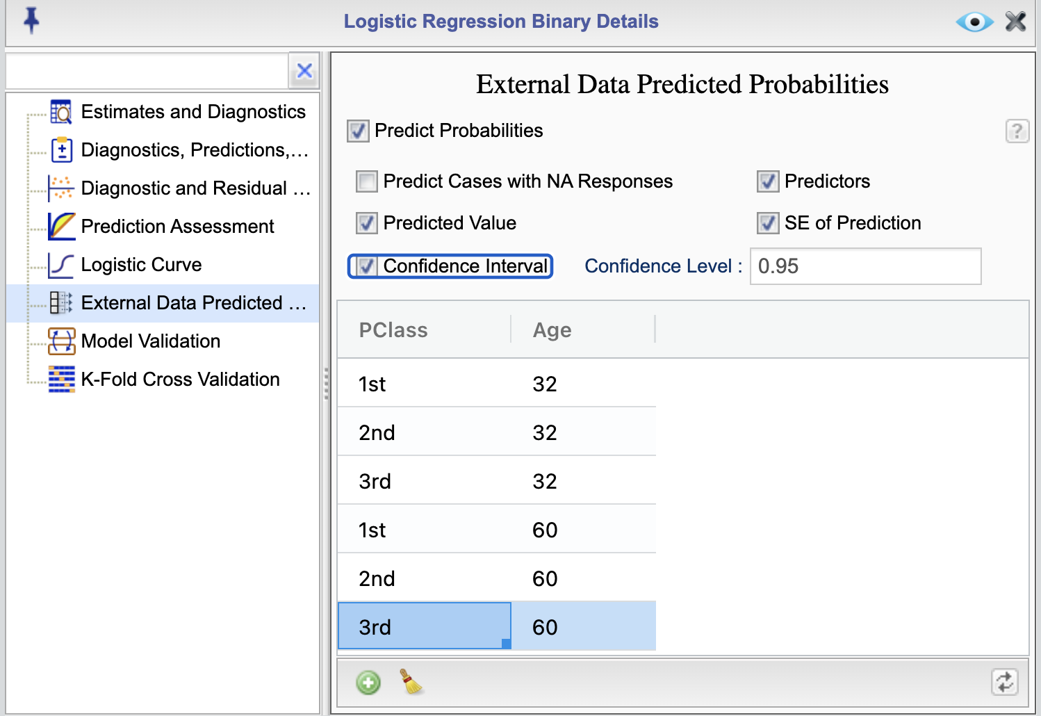
Figure 14.16: Predicted probabilities

14.13 An Example of Logistic Regression with Grouped Data

To illustrate an example of using Rguroo to fit logistic regression with grouped data, we use the orings dataset available in the Rguroo Users Guide dataset repository. These data are the 1986 Challenger disaster data that consists of information from 23 previous shuttle launches and includes the variables temperature in Fahrenheit (temperature), the number of O-rings that were damaged out of 6 (damaged), the number of O-rings that were not damaged (undamaged), and the number of trials (trials) which is equal to 6 in every case.

We Show how to use logistic regression in Rguroo to obtain the probability that an O-ring gets damaged as a function of the temperature.

14.14 K-Fold Cross Validation

You can use Rguroo’s K-Fold Cross-Validation function to assess your model performance. To access this option, click the Details button button in the Logistic Regression tab. This will open the Logistic Regression Details window. From there, select the K-Fold Cross Validation option to view the K-Fold Cross Validation dialog, shown in Figure 14.17. As shown in the figure, the K-Fold Cross Validation dialog includes two tabs. In the Fold Selection tab you can select options for partitioning the data to determine the folds, and in the K-Fold Report tab you can select options for the output.

To begin K-fold cross-validating, select the checkbox Start Validation. Note that you cannot apply the function K-Fold Cross-Validation and Cross-Validation at the same time.

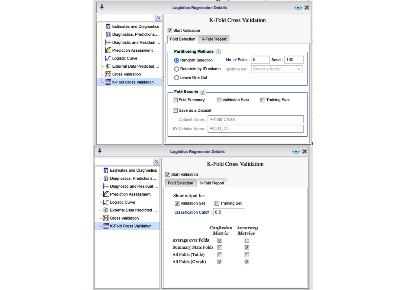
Figure 14.17: K-fold Fold Selection and Report dialog

14.14.1 Partitioning Methods

There are three methods of partitioning the data to create folds:

Random Selection: This method randomly partitions the data into your specified number of folds. You specify the number of folds in the No. of Folds textbox. The default value is 5. You can also specify a seed for the random number generation in the Seed textbox. The default value is 100.
Determine by ID Variable: This method partitions the data based on the levels of an ID variable. You can specify the ID variable by selecting a variable from the Partitioning Variable dropdown that includes the names of all categorical variables in the dataset. A fold consists of the cases corresponding to a level. If the ID variable of your choice is numerical, you can change its type to categorical in Rguroo’s Dataset Editor (see Section 2.3.5).
Leave-One-Out: This method partitions the data into the number of folds equal to the number of cases in the dataset. Each fold consists of one case. This method is equivalent to the jackknife method. The output report for this option is limited to a confusion matrix and a few accuracy metrics averaged over all folds, that can be shown for both validation and training sets, depending on the choice that you make in the K-Fold Report tab. The default is to show the average over the validation sets.

In the Fold Results section of the Fold Selection tab, there are three options: Fold Summary, Validation Sets, and Training Sets. These options provide, for each fold, a summary of number of cases, the case numbers for the validation set in each fold, and the case numbers for the training set in each fold.

You can save an ID variable that identifies the folds by selecting the Save as a Dataset checkbox in the Fold Results section. You need to specify a dataset name in the Dataset Name textbox and an ID variable name in the ID Variable Name textbox. Once you click the preview button, a Rguroo dataset, with the name you specify, will be created, including all the variables used in the model, with an ID variable column appended that identifies the folds. The saved dataset will be available under the Data toolbox.

14.14.2 K-Fold Report

In the K-Fold Report tab, you can select the output that you want to see for each fold. By default, the output will be based the validation sets, but you can also choose to see the output based on the training sets. You can make these choices by selecting one or both of the Validation Set and Training Set checkboxes. The following are the options available:

Confusion Matrix:
- Average over Folds : This option provides the average confusion matrix over all folds.
- Summary Stats Folds: This option provides the five-number summary plus the mean for the confusion matrix over all folds.
- All Folds (Table): This option provides the confusion matrix for each fold.
- All Folds (Graph): This option displays a graphical display of the confusion matrix for each fold.
Accuracy Metrics:
- Average over Folds : This option provides the average accuracy metrics over all folds.
- Summary Stats Folds: This option provides the five number summary plus the mean for the accuracy metrics over all folds.
- All Folds (Table): This option provides the accuracy metrics for each fold.
- All Folds (Graph): This option provides a graphical display of the accuracy metrics for each fold.

14.14.3 Fitting the model

Instructions for fitting a Logistic Regression model in Rguroo:

Recreate the example below by importing the orings dataset from the Rguroo Users Guide dataset repository into your account.

Click here to see a portion of the dataset.

Screenshot of the first 5 rows of the modified Oring dataset.

On the left-hand side of the Rguroo window, open the Analytics toolbox. Use the Analysis dropdown menu and choose Logistic Regression —> Grouped Data. The Logistic Regression Basics dialog will appear (see Figure 14.18).
Select a Dataset; for this example, the orings dataset.
In the Model Specification section, complete the following:
- Select the variable indicating the number of events from the Event dropdown; in this example, the variable damaged.
- Specify the variable that includes the number of non-events from the Non-Event dropdown; in this example, the variable undamaged.
- Note that alternatively you can select the variable trials, that includes the total number of trials (damaged + undamaged), from the Trial dropdown instead of either the variable damaged or undamaged .
- In the Model Formula textbox, specify the predictors. Predictors must be separated by a + sign. To get a model without an intercept, add -1 to your formula. See R documentation for details on how to specify models with interactions using “*” and “:”. For this example, we use temperature.
- From the Link dropdown, select the link function. The default is the logistic link function.
In the Event Label textbox, type a label for the event. In this example, we use “Damaged O-ring”
In the Non-Event Label textbox, type a label for non-event(s). In this example we use “Undamaged O-ring”
(Optional) Click the to add or modify output.
Click the Preview icon to view the result.

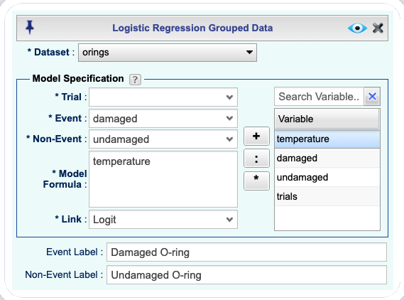
Figure 14.18: Logistic Regression Basics dialog

The Rguroo output is shown above. The output includes the following sections:

Data, Method, and Model, including the number of observed and missing data
Response Information, including the number of events and non-events
Parameter Estimates, including the estimated coefficients, standard errors, z-values, and p-values
Odds Ratios, including the odds ratios and their confidence intervals
Measures of Model Fit, including Deviance, Log-Likelihood, MSE, R-Squared, AIC, and BIC
Goodness of Fit Test, including Deviance, Pearson, and Hosmer-Lemeshow tests
Confusion Matrix, including True Positive, True Negative, False Positive, and False Negative counts and percentages.
ROC Plot and Cost Function Plot, including the ROC curve and the cost function plot, including the area under the curve (AUC) and optimal classification cutoff.