15 Linear Regression

You can fit linear regression models in Rguroo using three different functions:

To fit a simple regression model (with one predictor variable), use the Simple Regression function under the Analytics toolbox from the Linear Regression dropdown menu (see Chapter 14).
For general simple and multiple regression models, you can use either:
- the Simple & Multiple Regression function within the Linear Regression dropdown menu under the Analytics toolbox, or
- the Linear Regression function under the Prediction-Classification toolbox.

For regression modeling—including diagnostics, model selection, and advanced fitting methods—we recommend using the Linear Regression function under the Prediction-Classification toolbox. This function offers an extensive superset of features compared to the Simple & Multiple Regression function in the Analytics toolbox.

The instructions in this chapter focus on the Linear Regression function with the Least Squares option from the Prediction-Classification toolbox. These instructions also apply to the Simple & Multiple Regression function in the Analytics toolbox where features overlap.

Rguroo’s Linear Regression function supports fitting linear regression models—including simple and multiple regression—using least squares, bootstrap, ridge regression, and lasso methods. It also includes options for model selection, hypothesis testing, diagnostics, predictions, and performance evaluation (including k-fold cross-validation) when using the least squares method. This chapter describes these features in detail.

To begin, access the Linear Regression methods from the Prediction-Classification toolbox by following the click sequence Analysis –> Linear Regression and selecting one of the following functions:

Least Squares: Fits linear regression models using the least squares method, with a wide range of features including diagnostics, model selection, and more.
Bootstrap: Fits linear regression models using the bootstrap method.
Bootstrap Prediction: Generates predictions from a linear regression model fitted using the bootstrap method.
Ridge Regression: Fits linear regression models using the ridge regression method.
Ridge Prediction: Generates predictions from a linear regression model fitted using the ridge regression method.
Lasso Regression: Fits linear regression models using the lasso regression method.

All these functions share a common Basics dialog, with minor differences. Each allows you to specify the dataset, response variable, model formula, and weights (if applicable). However, the Details dialog differs for each function. This chapter describes the Details dialog for the least squares method. Subsequent chapters cover the Details dialog for the bootstrap, ridge regression, and lasso regression methods.

15.1 Linear Regression Basics Dialog

The Basics dialog for the Linear Regression functions is shown in Figure 15.1. This dialog allows you to specify your dataset, response variable, regression model using your predictors, and weights if applicable.

To get Rguroo’s default output using the Basics dialog, follow these steps:

Select a dataset from the Dataset dropdown menu.
Once you select a dataset, the variables from your dataset will appear in the Variable column on the right-hand side of the dialog. Also, the Response dropdown will populate with names of numerical variables from your selected dataset.
Select your response variable from the Response dropdown menu.
In the Model Formula textbox, specify your regression model see section 15.1.1 for more details.
If you are performing a weighted regression, select your weight variable from the Weight dropdown.
Click the preview icon to preview the results.

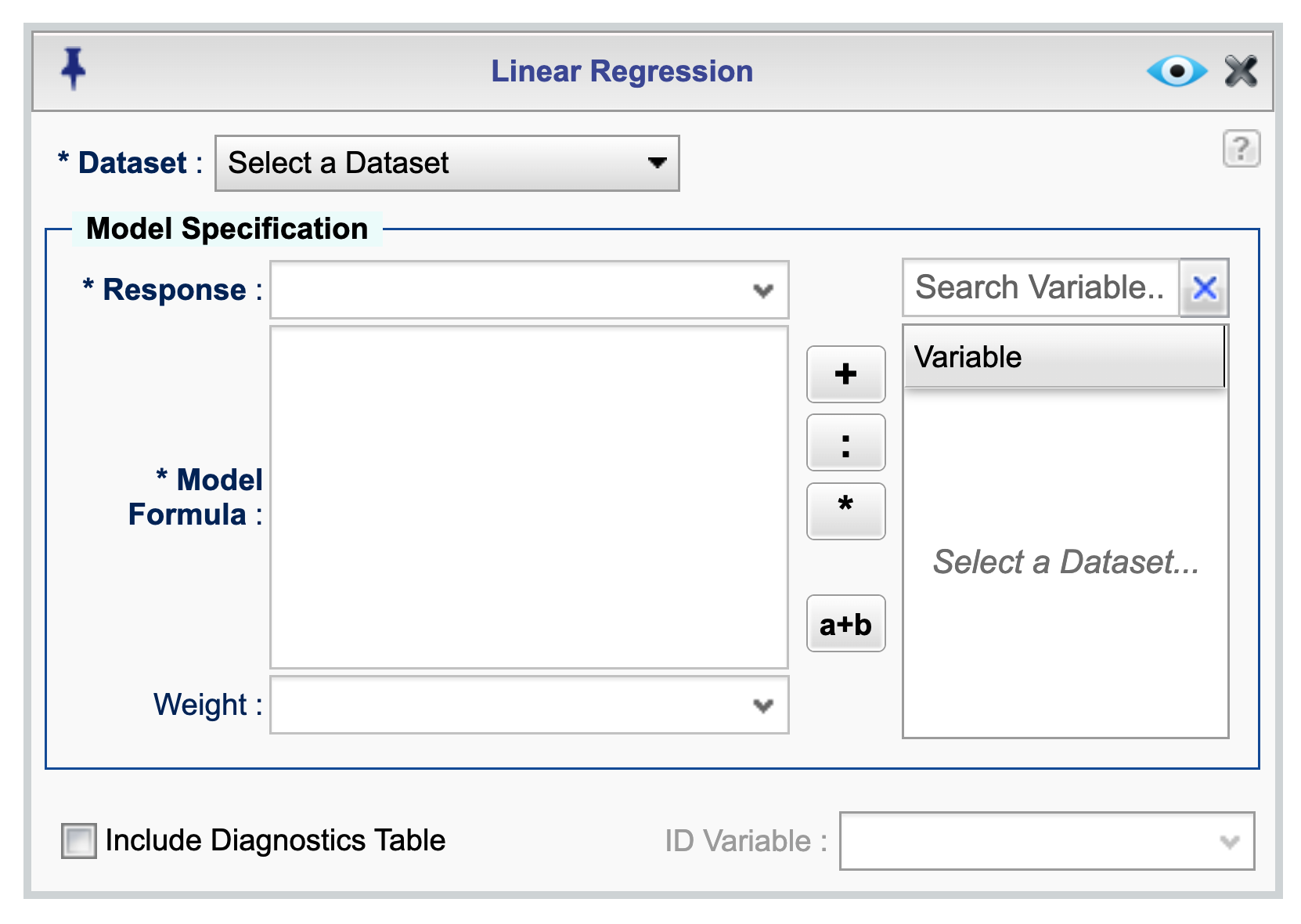
Figure 15.1: Linear Regression Basics dialog

15.1.1 Specifying your model in the model formula textbox

To specify your model, you can either type variable names directly into the Model Formula textbox or double-click variable names from the Variable column to insert them automatically. Depending on your model, use one of the following operators to separate variable names: +, *, or :.

An additional operator, a+b, allows you to select multiple variables and add them together at once. To use it, select multiple variables and click the a+b button—this will insert all selected variables into the formula with plus signs between them. This feature is especially useful when you want to include many variables in the model quickly.

To fit a model without an intercept (forcing the intercept to zero), add -1 to your formula. For example:

Model with intercept: x1 + x2
Model without intercept: x1 + x2 - 1

To specify interactions between predictors, use * or :. For example:

Interaction with main effects: x1 * x2
Interaction-only term: x1 + x2 + x1:x2

For more details on specifying model formulas in R, see R documentation for Model Formulae.

15.1.2 Default Output using the Basic Dialog

When you click the Preview icon for one of the the Linear Regression functions, Rguroo generates a comprehensive output that includes the results of the linear regression analysis. By default, the output from the Linear Regression function generally includes:

The method used for estimation.
A summary of the dataset used for the analysis.
The model formula specified.
Regression coefficients, including estimates, standard errors, t-values, and p-values.
R-squared and adjusted R-squared values.
ANOVA table for the model.
a residuals vs. fitted values plot.
A normal probability plot of the residuals.

15.1.3 Fitted values and predictions in the Basics dialog

Generally, the fitted values and predictions can be obtained in the Details dialog for various fitting methods. However, for the least squares method specifically, an additional option, Include diagnostics, is available in the Basics dialog. If you select the Include diagnostics checkbox in the dialog, the output will also include a table with columns including the response variable, the residuals, Cook’s distance, and Leverage (Hat values). Additionally, if you select a variable from the ID variable dropdown, the output table will include a column with the values of that variable. You can obtain other diagnostics in the details dialog by clicking the Details button button. See sections 15.4 for more details on the available diagnostics.

15.2 Polynomial Regression

You can fit polynomial regression models using the Linear Regression function in Rguroo. To fit polynomial regression models, use the poly() function directly within the Model formula textbox.

For example, to specify a quadratic polynomial (second-degree) for a predictor x, enter: poly(x, degree = 2, raw = TRUE).
For higher-order polynomials, simply adjust the degree parameter.
To use orthogonal polynomials (recommended for better numerical stability), set raw = FALSE: For example, poly(x, degree = 2, raw = FALSE).

For more details, refer to the R documentation on poly R documentation for the poly() function.

An alternative to using the poly() function is to use the I() function to specify polynomial terms directly in the model formula. For example, to fit a third degree polynomial, you can enter x + I(x^2) + I(x^3) in the Model formula textbox.

15.3 Details for Least Squares Regression

The Linear Regression function in Rguroo provides a comprehensive set of features for fitting and evaluating linear regression models when using the least squares method. These features can be accessed by clicking the Details button button at the top of the application. Clicking this button opens the Details dialog, which allows you to select additional output options and advanced features for your regression analysis. Figure 15.2 shows the Details dialog for liner regression’s Least squares function. Through this dialog you can access a range of options for model fitting, model evaluation, model selection, and prediction.

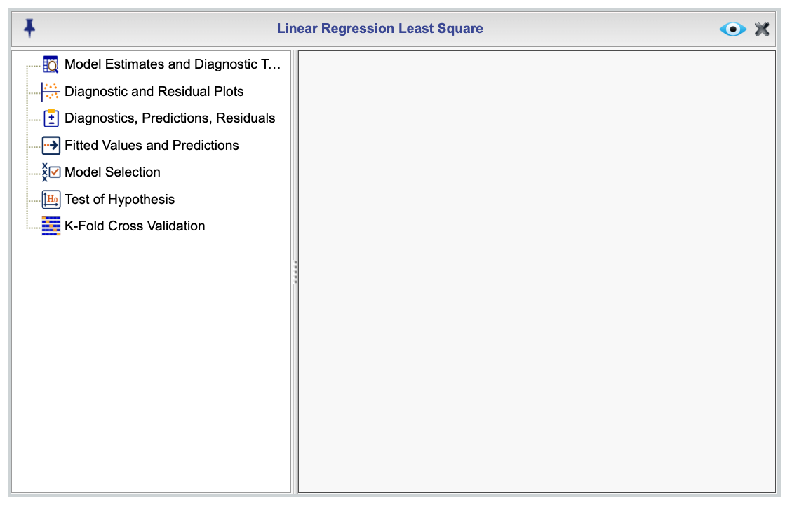
Figure 15.2: Linear Regression Least Squares Details dialog

15.4 Model Estimates, Predictions, Diagnostics Indices and Graphs

In the Details dialog of the Least Squares function, there are four sections dedicted to requesting additional output related to model estimates, predictions, diagnostics indices, and graphs. The following subsections describe these sections in detail.

15.4.1 Model Estimates and Diagnostics Tables

Figure 15.3 shows the Model Estimates and Diagnostics Table section of the Details dialog, along with its available options. This section allows you to select from a variety of tables including indices related to model estimates and diagnostics.

In the figure, the names listed in the Selected column are the default tables that will be included in the output. You can deselect all selected items by clicking the Deselect All button, and restore the default selections by clicking the Default button. To include a new table, simply drag its name from the Options column to the Selected column or use the arrow keys. You can also reorder the selected tables by dragging them up or down within the Selected column.

The textbox Confidence Level lets you specify the confidence level for the Parameter Confidence Interval output. The default value is 0.95, corresponding to a 95% confidence level. You can change this to any number between 0 and 1.

The textbox No. of Decimal Places allows you to specify the number of decimal places to display in the output tables. If left blank, Rguroo will choose a reasonable default. If you enter an integer value greater than or equal to 0, that number of digits after the decimal point will be used in output tables that includes values with decimals.

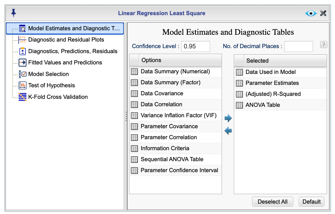
Linear Regression Model Estimates and Diagnostics Table dialog

Figure 15.3: Model Estimates and Diagnostics Table dialog

15.4.2 Model Estimates and Diagnostics Plots

Figure 15.4 shows the Diagnostics and Residual Plots section of the Details dialog, along with its available options. This section allows you to select from a variety of graphs related to model estimates and diagnostics.

The Selected column in the figure shows the default graphs that will be included in the output. You can deselect all selected items by clicking the Deselect All button, and restore the default selections by clicking the Default button. To include a new graph, simply drag its name from the Options column to the Selected column. You can also reorder the selected graphs by dragging them up or down within the Selected column.

The textbox Confidence Level lets you specify the confidence level for the graph corresponding to the selection Prediction band. When this option is selected, corresponding to each predictor, a scatterplot with its horizontal access being a predictor value and its vertical access being the response will be plotted along with the least squares line and a confidence band. The default value for the confidence band is 0.95, corresponding to a 95% confidence level. You can change this to any number between 0 and 1.

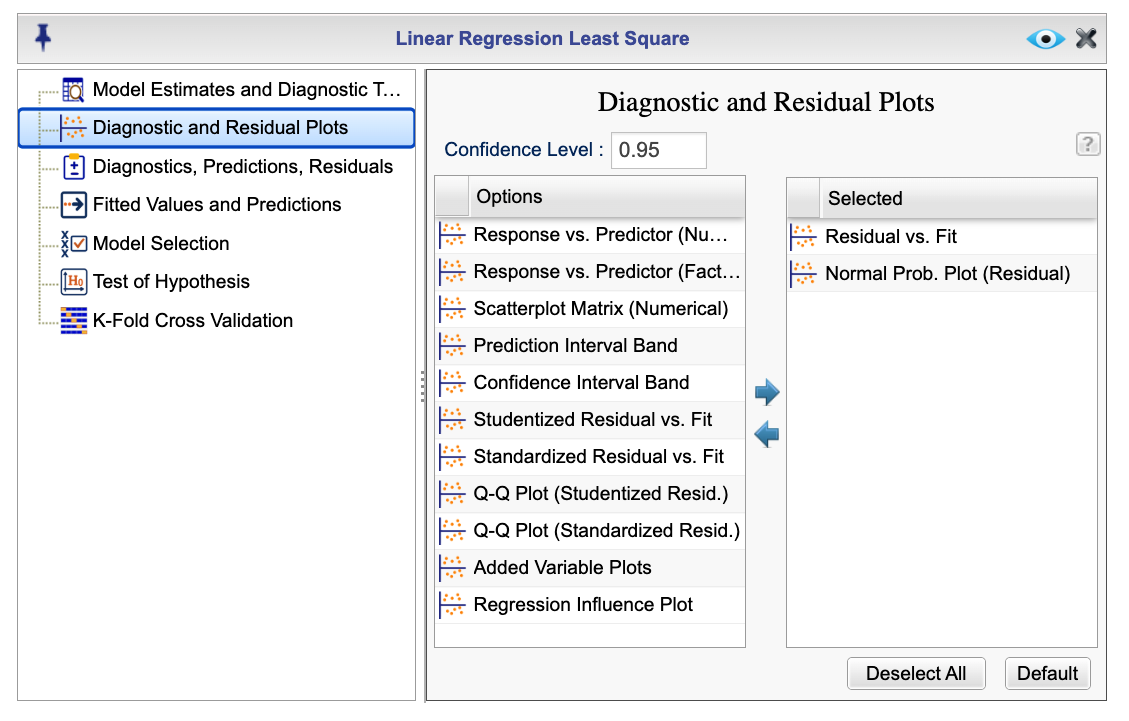
Linear Regression Model Diagnostics and Residual Plots dialog

Figure 15.4: Diagnostic and Residual Plots dialog

15.4.3 Diagnostics, Predictions and Residuals

Figure 15.5 shows the Diagnostics, Predictions and Residuals section of the Details dialog, along with its available options. To begin, you select the Create Table checkbox. When the Create Table checkbox is selected, the Diagnostics, Predictions, Residuals section becomes active, allowing you to obtain fitted values, residuals, and a variety of diagnostics indices, .

By default the option Load Table into Viewer is selected, which means that the output table will be displayed in the Rguroo viewer. Once the table is loaded in the viewer, you have various options to filter and sort the table, as well as to save it as an Rguroo dataset. You can also export the table to a CSV or Excel file by right-clicking on the table. By selecting the Include Table in Report checkbox, you can also include the table in the Rguroo report.

The Selected column in the figure shows the default diagnostics indices that will be included in the output. You can deselect all selected items by clicking the Deselect All button, and restore the default selections by clicking the Default button. To include a new index, simply drag its name from the Options column to the Selected column. You can also reorder the selected indices by dragging them up or down within the Selected column.

The textbox No. of Decimals allows you to specify the number of decimal places to display in the output tables in the report. If you enter an integer value greater than or equal to 0, that number of digits after the decimal point will be used consistently in all output tables. If left blank, Rguroo will choose a reasonable default. You can also specify an ID variable to be included in the output table. This variable will be displayed as the first column of the table and can be used to identify each row in the table.

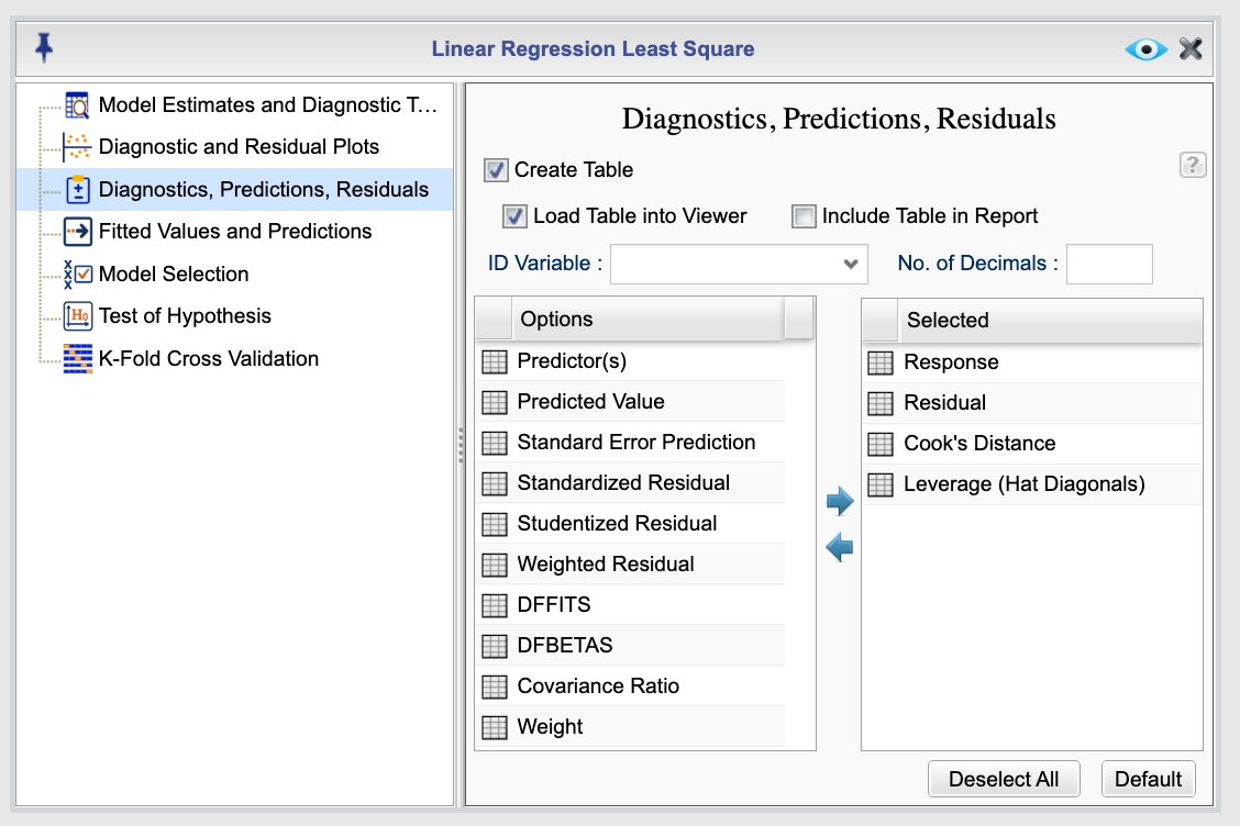
Linear Regression Model Diagnostics fitted values and Residual Plots dialog

Figure 15.5: Diagnostic, Fiited Values, and Residuals dialog

15.4.4 Fitted values and external data predictions, including prediction intervals

Figure 15.6 shows the Fitted Values and Prediction section of the Details dialog, along with its available options. This section allows you to select from various fitted value and prediction outputs, including predicted values, standard errors of the predictions, standard error of prediction, confidence intervals for the mean prediction, and prediction intervals. You can also specify an ID variable to be included in the output table—this variable will serve to identify each row in the output. This dialog can also be used to make predictions for new cases, either from the main dataset or from an external dataset.

To obtain fitted values and predictions, select the Show Predictions checkbox. When this checkbox is selected, the Fitted Values and Prediction section becomes active, allowing you to obtain fitted values and predictions for the cases used to fit the model or for external data.

You can specify confidence level for the confidence intervals and prediction intervals using the Confidence Level textbox. The default value is 0.95, corresponding to a 95% confidence level. You can change this to any number between 0 and 1. You can also specify the number of decimal places to display in the output tables using the No. of Decimal Places textbox. If you enter an integer value greater than or equal to 0, that number of digits after the decimal point will be used consistently in all output tables. If left blank, Rguroo will choose a reasonable default. Note that the number of decimal places specified will be used for the table that appears in the Rguroo report. The table that appears in the Rguroo viewer (see below)will have the maximum number of decimals for computation purposes.

Internal Data and External Data:

If you check the Load Table into Viewer checkbox next to Internal Data, the fitted values (i.e., predictions) for the cases used to fit the model will be computed and loaded into the viewer.
If you check the Load Table into Viewer checkbox next to External Data, predictions will be generated for data not used in model fitting.

Below, we show two methods for specifying external data. In both cases, the predicted values will appear in the viewer. The viewer can be used to filter, sort, and save the data as an Rguroo dataset. You can also export the table as a CSV or Excel file from the viewer by right-clicking on the dataset.

If you check the Include Table in Report checkboxes next to Internal Data or External Data, the corresponding prediction tables will be included in the Rguroo report.

There are two ways to specify external data in Rguroo:

Using the main dataset:
Add external cases directly to the dataset used to fit the model, and set their response variable values to NA. Then check the Predict Cases with NA response box to generate predictions for these cases. Rguroo will treat all cases with NA responses as new observations and compute predictions for them.
Using the built-in dataset editor:
After specifying a model, the dataset editor at the bottom of the dialog will display the names of the variables used in your model. You can manually enter values for new cases here:
- For numerical variables, type in the desired values.
- For categorical variables (factors), click a cell to display a dropdown list of available levels.
By default, the editor shows 5 rows, but you can add more by clicking the plus icon at the bottom of the editor. If you update the model and the variables are not appearing, click the refresh icon to reload the variable list.

Linear Regression fitted values predictions, and prediction interval dialog

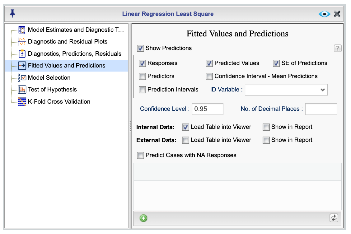
Figure 15.6: Fitted values, predictions, and prediction intervals dialog

15.5 Model Selection

You can use the Model Selection dialog in Rguroo’s Linear Regression function for variable selection. Figure 15.7 displays the Model Selection dialog, which is accessible via the Details dialog of the Linear Regression function. This dialog enables you to specify a model selection method and criterion, as well as other options to customize the selection process.

To begin model selection, you must first specify a model in the Basics dialog. Then in the Model Selection dialog select the checkbox Select Models. This activates the model selection options.

From the Selection Method dropdown, you can choose one of the following model selection method: Stepwise (bidirectional), Backward, Forward, and Best Subset. The default method is Stepwise. For each method , you can select a criterion for model selection from the Selection Criterion dropdown. The available criteria include AIC, BIC, R-Square, Adjusted R-Square, Mallow’s Cp, and P-Value. The default criterion is AIC.

If you select the Best Subset method, the Options button will be enabled, allowing you to specify additional options for the best subset selection. The default output for the best subset method is to display the best model among all models based on the selected criterion. Other options are Best p-variable model, All in order of number of covariates, and All sorted by selected criteria.

When you choose P-Value as your selection criterion, you can specify P-value to Enter and P-value to Remove thresholds. The default values are 0.05 for entering and 0.1 for removing variables. These thresholds can be adjusted. The P-Value to Enter threshold determines the significance level at which a variable is added to the model, while the P-Value to Remove threshold determines the significance level at which a variable is removed from the model. The P-Value to Enter must be smaller than the P-Value to Remove.

The Forced Variables section allows you to specify any variables that must be included in the model, regardless of their significance. Once you specify a model and activate the Model Selection dialog, the Variables column is populated with the variables in the model. You can select the variables that you want to force their inclusion in the model by dragging them to the Forced Variables column. These variables will be included in all selected models.

Note that a maximum of 256 models can be fit for evaluation. If the number of models exceeds this limit, Rguroo will display a warning message and only the first 256 models will be evaluated.

If you click on the No. of Decimal Places button, a dialog will open allowing you to specify the number of decimal places to display in the output tables for parameter estimates, R-squared and Adjusted R-squares, and AIC, BIC, and Cp values.

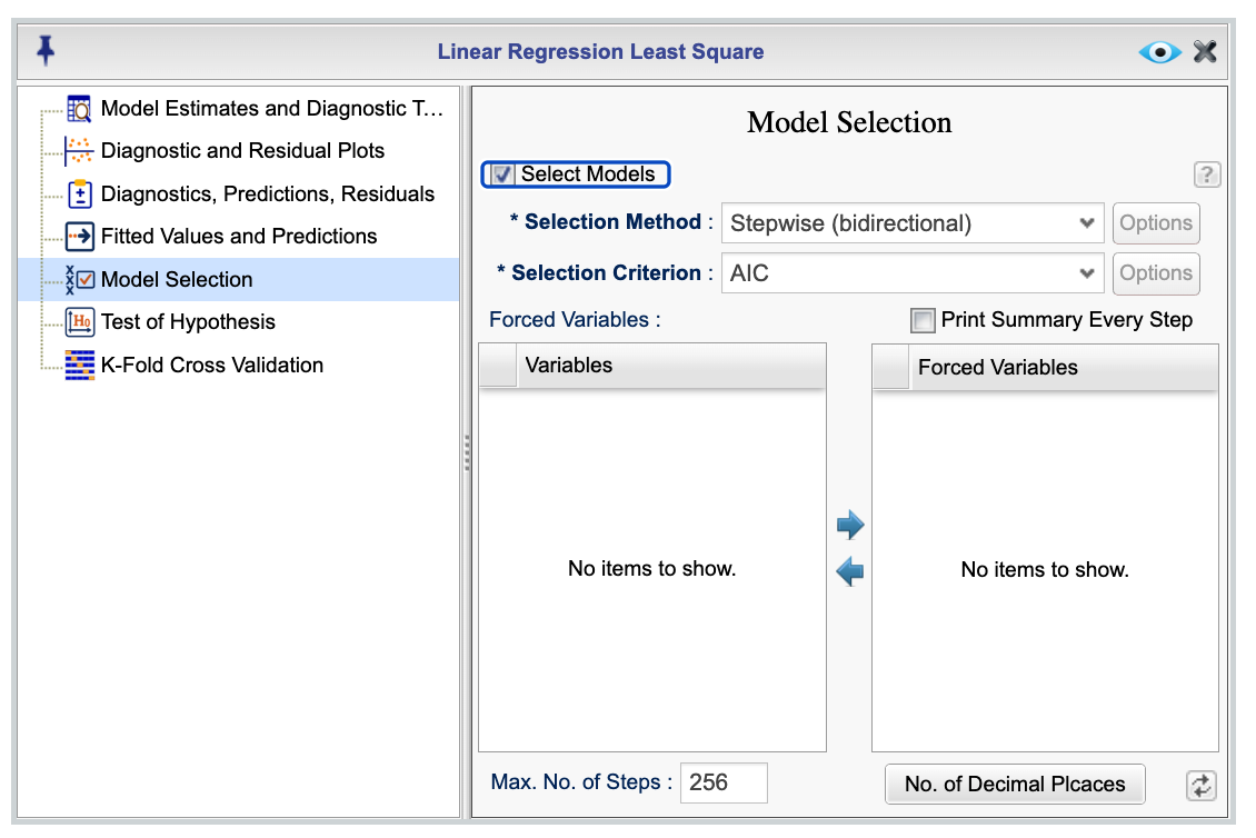
Linear Regression model selection dialog

Figure 15.7: Model Selection dialog

15.6 Testing Nested Models and Contrast Hypotheses

In Rguroo, you can test nested models and contrast hypotheses using the Test of Hypothesis dialog, which is accessible through the Details dialog of the Linear Regression function. Figure 15.8 shows the Test of Hypothesis dialog that consists of two tabs labeled Nested Models and Contrasts.

15.6.1 Testing Nested Models

The tab being shown in the Figure 15.8 is the Nested Model interface that allows you to test models that are nested within the full model specified in the Basics dialog. On the left-hand side, you will see the list of parameter names corresponding to the full model. In the example shown, parameter names from a model using the cardata dataset, available in the Rguroo dataset repository, are displayed.

To define a hypothesis test, begin by entering a name in the first row of a column. By default two columns labeled Hypothesis 1 and Hypothesis 2 are created. You can change these names as you desire. Once a name is entered, all rows in that column will be checked by default, indicating that the corresponding variables are included in the model for that hypothesis. If all variables are checked, no hypothesis will be tested. To specify a nested model, relative to the full model, simply uncheck the checkboxes corresponding to the model parameters you want to exclude.

The nested model you define this way will be tested against the full model. You can create and test multiple hypotheses by adding more columns using the plus icon at the bottom of the dialog. F-test will be used to test the nested models, and the results will be displayed in the output table. The output will include the F-statistic, degrees of freedom, and p-value for each hypothesis test.

If you change your full model, you can use the refresh icon to reload the parameter names corresponding to the new full model. This will update the list of parameters in the left-hand side of the dialog.

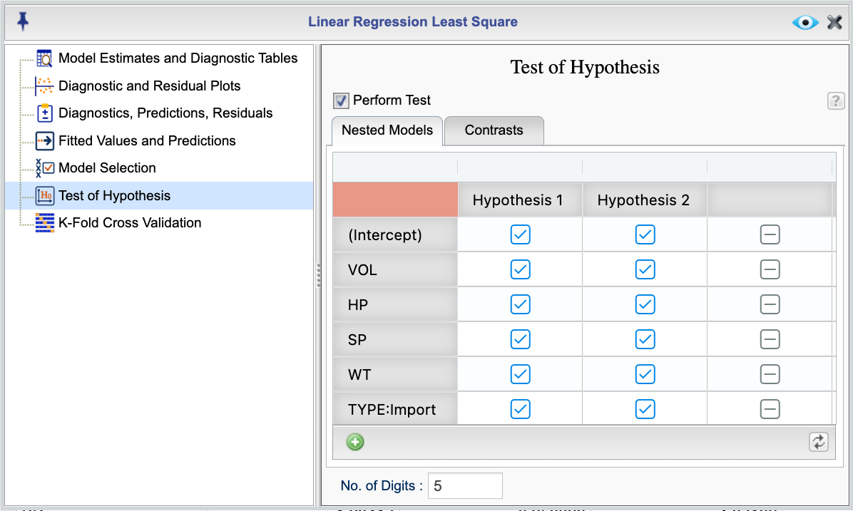
Figure 15.8: Test of hypothesis dialog for testing nested models

15.6.2 Testing Contrasts

In Rguroo, you can test contrasts between levels of a factor variable in your model or any linear combination of model parameters using the Test of Hypothesis dialog, which is accessible through the Details dialog of the Linear Regression function.

Figure 15.9 shows the Contrasts tab of the Test of Hypothesis dialog. This tab allows you to test contrasts between levels of a factor variable in your model or any linear combination of model parameters. As in the nested model testing tab, the left-hand side of the dialog lists all parameters corresponding to the full model. In the figure shown, the parameters from a model using the cardata dataset, available in the Rguroo dataset repository, are listed. To define a contrast, start by entering a name in the first row of a column. Once a name is entered, you can specify the contrast by entering numerical values in the rows of that column.

The last row of the first column, labeled Equation RHS, is reserved for the Right-Hand Side (RHS) of the contrast equation, which is typically set to 0. The other rows contain the coefficients for each parameter in the contrast. By default, all values are initialized to 0, indicating that no contrast is specified.

For example: - To test the contrast x1 - x2 = 0, enter 1 for x1, -1 for x2, and 0 in the RHS row. - To test the hypothesis x1 + 2 * x2 = 5, enter 1 for x1, 2 for x2, and 5 in the RHS row.

You can also test multiple contrasts simultaneously by assigning the same name to each column. For instance, to jointly test x1 - x2 = 0 and x3 - x4 = 0, do the following: 1. Enter a name like Contrast1 in the first row of a new column and set the coefficients for x1 and x2, with 0 in the RHS row. 2. In another new column, also name it Contrast1, and set the coefficients for x3 and x4, again with 0 in the RHS row.

By assigning the same name to both columns, Rguroo will test the two contrasts together as a joint hypothesis.

You can add additional contrasts by clicking the plus icon at the bottom of the dialog.

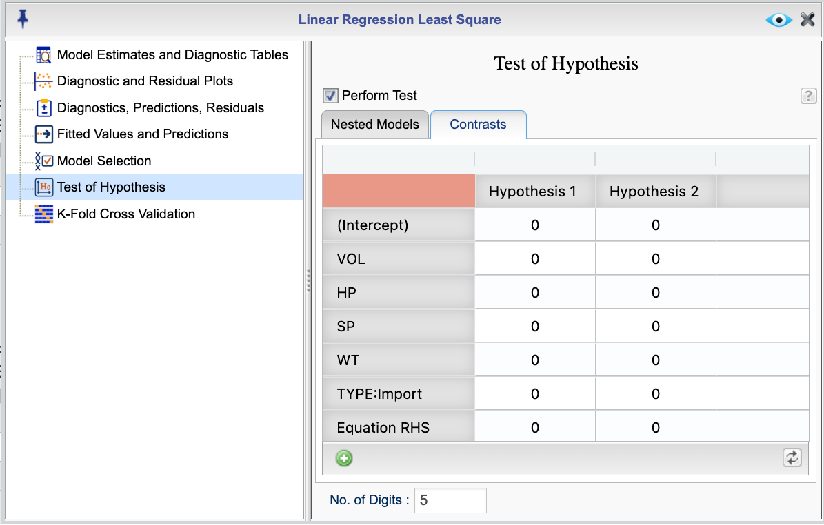
Figure 15.9: Test of hypothesis dialog for testing contrasts

15.7 K-Fold Cross-Validation

You can perform k-fold cross-validation using the Linear Regression function in Rguroo. This option is available through the Details dialog and enables you to assess the predictive performance of your regression model.

Figure 15.10 displays the K-Fold Cross-Validation dialog, which contains two tabs: Fold Selection and K-Fold Report.
- The Fold Selection tab lets you specify the number of folds and choose a method for assigning observations to folds. In this tab you can also ask for fold summaries and request to see the folds in the viewer.

The K-Fold Report tab allows you to request various statistics and outputs from the cross-validation process.

15.7.1 The Fold Selection Tab

In the Partitioning Methods section of the Fold Selection tab, you can choose one of the following fold selection methods:

Random Selection: Randomly assigns cases to folds. You can specify the number of folds in the No. of Folds textbox. The default is 5, but you may enter any reasonable positive integer. You can also set a random seed in the Seed textbox to ensure reproducibility.
Determine by ID column: Assigns folds based on a splitting variable that you select from the Splitting Var dropdown. This dropdown lists all factor (categorical) variables in your dataset. If you want to use a numerical variable as a splitting variable, you can change its type to a factor in the Rguroo dataset editor.
Leave One Out: Uses each individual case as its own fold, performing leave-one-out cross-validation.

In the Fold Results section of the Fold Selection tab, you can request the following:

Fold Summaries: Displays a summary for each fold, including the number of training cases and the number of validation cases.
Validation Sets: Displays the observations included in each validation set for all folds.
Training Sets: Displays the observations included in each training set for all folds.
Load K-Fold Cross Validation Dataset to Viewer: Loads the K-Fold Cross Validation dataset into the viewer for further inspection. This dataset contains all variables used in the model plus an additional column, added as the last column, with the default name FOLD_ID. You can specify a custom name for this fold ID column in the ID Variable Name textbox. This column identifies the fold number for each observation (e.g., Fold1, Fold2, etc.), making it easy to see which observations belong to which folds. In the viewer, you can filter and save the dataset that includes the fold IDs for further analysis.

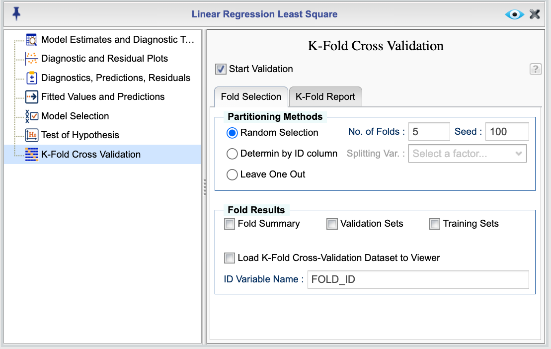
Figure 15.10: Dialog for fold Selection for K-fold cross validation

15.7.2 The K-Fold Report Tab

Figure 15.11 shows the K-Fold Cross-Validation Report dialog, accessible through the Details dialog of the Linear Regression function. This dialog lets you configure how the results of the k-fold cross-validation are displayed.

In the Performance Metrics section, you can request the following metrics: Root Mean Square Error (RMSE), Mean Absolute Error (MAE), Mean Absolute Percent Error (MAPE), R-square, and Prediction Correlation (correlation between predicted and observed values).

You can choose from the following options:

Summary: Displays the five-number summary (minimum, first quartile, median, third quartile, maximum) and the mean for each performance metric across validation folds.
All Folds: Displays individual performance metrics for each fold.
Metrics Graph by Fold: Displays a graph showing the performance metrics across all folds.

You can also select the Graph of Predicted vs. Observed option to display a graph of predicted versus observed response values for each fold. This graph is shown by default.

By default, all selected metrics are reported for the validation set. To view metrics for the training set, check the Training Set checkbox.

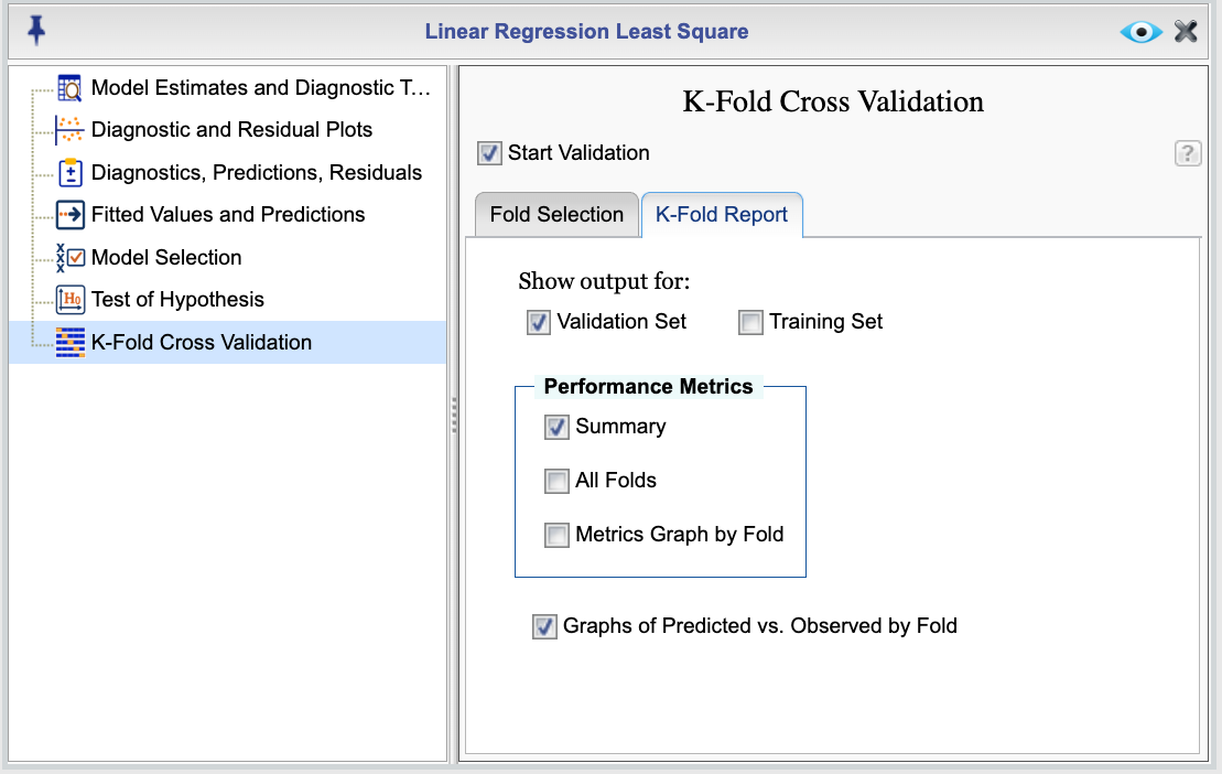
Figure 15.11: K-fold cross validation report dialog

15.8 Examples of Linear Regression with Least Squares Estimation Methods

15.8.1 An Example of Fitting a Multiple Regression Model Using Least Squares

Instructions for fitting a multiple linear regression model in Rguroo:

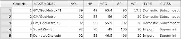
Use a dataset in your Rguroo account or recreate the example below by importing the cardata dataset from the Rguroo dataset repository called Rguroo Users Guide into your account.

Click here to see a portion of the dataset.

Screenshot of the first 5 rows of the Cardata dataset.

Open the Analytics toolbox on the left-hand side of the Rguroo window. Use the Analysis dropdown menu and choose Linear Regression —> Simple & Multiple Regression. This will open the Multiple Regression dialog box (see Figure 15.12).
Select a Dataset.
In the Model Specification section, select your response variable from the Response drop down.
In the formula textbox, add your predictors. Predictors must be separated by a + sign. To get a model without an intercept, add -1 to your formula. See R documentation for details on how to specify models with interactions using “*” and “:”.
(Optional) Click the to add additional output, including model estimate and diagnostics graphs, diagnostic indices, fitted values, and prediction intervals.
Click the Preview icon to view the result.

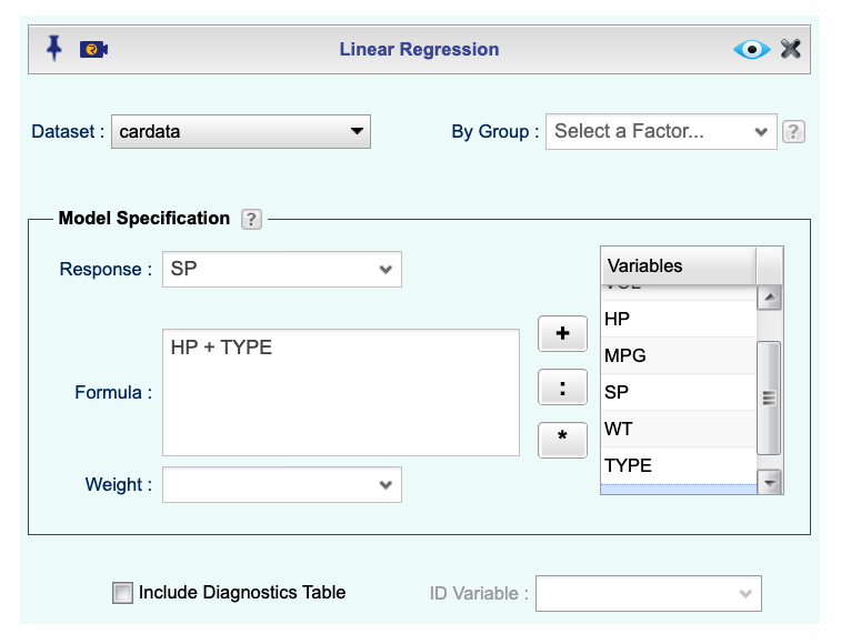
Figure 15.12: Multiple regression dialog

15.8.2 An example of Regression Prediction Intervals

Instructions for obtaining prediction intervals in Rguroo:

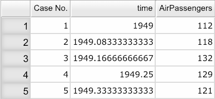
Use a dataset in your Rguroo account or recreate the example below by importing the AirPassengers dataset from the Rguroo dataset repository called R datasets into your account.

Click here to see a portion of the dataset.

Screenshot of the first 5 rows of the Air Passenger dataset.

Open the Analytics toolbox on the left-hand side of the Rguroo window. Use the Analysis dropdown menu and choose Linear Regression —> Simple & Multiple Regression. This will open the Multiple Regression dialog box (see Figure 15.13).
Select a Dataset.
In the Model Specification section, select your response variable from the Response dropdown.
In the formula textbox, add your predictors. Predictors must be separated by a + sign. To get a model without an intercept, add -1 to your formula. See R documentation for details on how to specify models with interactions using “*” and “:”.
Click the and select the Fitted Values, Predictions, and Interval Estimates tab. Here, move Prediction Interval to the Selected column using drag-and-drop or the menu arrows.
Check one or both of the options Internal Data or External Data. Internal data refers to cases that are used to fit the model. External data refers to cases that are not used to fit the model. You specify the external data by adding them to your dataset and setting the response variable column for these cases to NA.
Click the Preview icon to view the result.

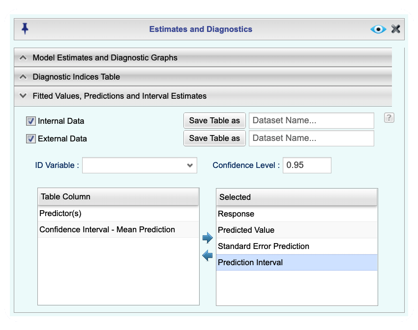
Figure 15.13: Regression Prediction Intervals dialog